HyperSQL Database Engine 2.7.4
|
2024-10-25 |
|
Table of Contents
- Preface
- 1. Running and Using HyperSQL
- 2. SQL Language
-
- SQL Standards Support
-
- Definition Statements (DDL and others)
- Data Manipulation Statements (DML)
- Data Query Statements (DQL)
- Calling User Defined Procedures and Functions
- Setting Properties for the Database and the Session
- General Operations on Database
- Transaction Statements
- Comments in Statements
- Statements in SQL Routines
- SQL Data and Tables
- Short Guide to Data Types
- Data Types and Operations
- Datetime types
- Interval Types
- Arrays
- 3. Schemas and Database Objects
-
- Overview
- Schemas and Schema Objects
- Statements for Schema Definition and Manipulation
-
- Common Elements and Statements
- Renaming Objects
- Commenting Objects
- Schema Creation
- Table Creation
- Temporal System-Versioned Tables and SYSTEM_TIME Period
- Table Settings
- Table Manipulation
- View Creation and Manipulation
- Domain Creation and Manipulation
- Trigger Creation
- Routine Creation
- Sequence Creation
- SQL Procedure Statement
- Other Schema Objects Creation and Alteration
- The Information Schema
- 4. Built In Functions
- 5. Data Access and Change
- 6. Sessions and Transactions
- 7. Text Tables
- 8. Access Control
- 9. SQL-Invoked Routines
-
- Overview
- Routine Definition
- SQL Language Routines (PSM)
-
- Advantages and Disadvantages
- Routine Statements
- Compound Statement
- Table Variables
- Variables
- Cursors
- Handlers
- Assignment Statement
- Select Statement : Single Row
- Formal Parameters
- Iterated Statements
- Iterated FOR Statement
- Conditional Statements
- Return Statement
- Control Statements
- Raising Exceptions
- Routine Polymorphism
- Returning Data From Procedures
- Recursive Routines
- Java Language Routines (SQL/JRT)
- User-Defined Aggregate Functions
- 10. Triggers
- 11. System Management
-
- Modes of Operation
- Indexes and Query Speed
- Query Processing and Optimisation
- ACID, Persistence and Reliability
- Temporal System-Versioned Tables
- Replicated Databases
- Using Table Spaces
- Checking Database Tables and Indexes
- Backing Up and Restoring Database Catalogs
- Encrypted Databases
- Monitoring Database Operations
- Database Security
- Statements
- 12. Deployment Guide
- 13. Compatibility With Other DBMS
- 14. Properties
- 15. HyperSQL Network Listeners (Servers)
- 16. HyperSQL on UNIX
- 17. HyperSQL via ODBC
- A. Lists of Keywords
- B. HyperSQL Database Files and Recovery
- C. Building HSQLDB Jars
- D. HyperSQL with OpenOffice
- E. HyperSQL File Links
- SQL Index
- General Index
List of Tables
- 1. Available formats of this document
- 2.1. List of SQL types
- 4.1. TO_CHAR (number) format elements
- 4.2. TO_CHAR, TO_DATE and TO_TIMESTAMP format elements
- 14.1. Memory Database URL
- 14.2. File Database URL
- 14.3. Resource Database URL
- 14.4. Server Database URL
- 14.5. User and Password
- 14.6. Closing old ResultSet when Statement is reused
- 14.7. Column Names in JDBC ResultSet
- 14.8. In-memory LOBs from JDBC ResultSet
- 14.9. Empty batch in JDBC PreparedStatement
- 14.10. Automatic Shutdown
- 14.11. OpenOffice and Libre Office usage
- 14.12. Validity Check Property
- 14.13. Creating New Database Check Property
- 14.14. Execution of Multiple SQL Statements etc.
- 14.15. SQL Keyword Use as Identifier
- 14.16. SQL Keyword Starting with the Underscore or Containing Dollar Characters
- 14.17. Reference to Columns Names
- 14.18. String Size Declaration
- 14.19. Truncation of trailing spaces from string
- 14.20. Type Enforcement in Comparison and Assignment
- 14.21. Foreign Key Triggered Data Change
- 14.22. Use of LOB for LONGVAR Types
- 14.23. Type of string literals in CASE WHEN
- 14.24. Concatenation with NULL
- 14.25. NULL in Multi-Column UNIQUE Constraints
- 14.26. Truncation or Rounding in Type Conversion
- 14.27. Decimal Scale of Division and AVG Values
- 14.28. Support for NaN values
- 14.29. Sort order of NULL values
- 14.30. Sort order of NULL values with DESC
- 14.31. String Comparison with Padding
- 14.32. Default Locale Language Collation
- 14.33. Case-Insensitive Varchar columns
- 14.34. Lowercase column identifiers in ResultSet
- 14.35. Storage of Live Java Objects
- 14.36. Names of System Indexes Used for Constraints
- 14.37. DB2 Style Syntax
- 14.38. MSSQL Style Syntax
- 14.39. MySQL Style Syntax
- 14.40. Oracle Style Syntax
- 14.41. PostgreSQL Style Syntax
- 14.42. Maximum Iterations of Recursive Queries
- 14.43. Default Table Type
- 14.44. Transaction Control Mode
- 14.45. Default Isolation Level for Sessions
- 14.46. Transaction Rollback in Deadlock
- 14.47. Transaction Rollback on Interrupt
- 14.48. Interval Types
- 14.49. Temporary Result Rows in Memory
- 14.50. Opening Database as Read Only
- 14.51. Opening Database Without Modifying the Files
- 14.52. Event Logging
- 14.53. SQL Logging
- 14.54. Table Spaces for Cached Tables
- 14.55. Huge database files and tables
- 14.56. Use of NIO for Disk Table Storage
- 14.57. Use of NIO for Disk Table Storage
- 14.58. Internal Backup of the .data File
- 14.59. Unused Space Recovery
- 14.60. Rows Cached In Memory
- 14.61. Size of Rows Cached in Memory
- 14.62. Size Scale of Disk Table Storage
- 14.63. Size Scale of LOB Storage
- 14.64. Compression of BLOB and CLOB data
- 14.65. Use of Lock File
- 14.66. Logging Data Change Statements
- 14.67. Automatic Checkpoint Frequency
- 14.68. Automatic Defrag at Checkpoint
- 14.69. Compression of the .script file
- 14.70. Logging Data Change Statements Frequency
- 14.71. Logging Data Change Statements Frequency
- 14.72. Recovery Log Processing
- 14.73. Default Properties for TEXT Tables
- 14.74. Forcing Garbage Collection
- 14.75. Crypt Property For LOBs
- 14.76. Cipher Key for Encrypted Database
- 14.77. Cipher Initialization Vector for Encrypted Database
- 14.78. Crypt Provider Encrypted Database
- 14.79. Cipher Specification for Encrypted Database
- 14.80. Logging Framework
- 14.81. Text Tables
- 14.82. Java Functions
- 15.1. common server and webserver properties
- 15.2. server properties
- 15.3. webserver properties
- 17.1. Settings List
List of Examples
- 1.1. Java code to connect to the local hsql Server
- 1.2. Java code to connect to the local http Server
- 1.3. Java code to connect to the local secure SSL hsqls: and https: Servers
- 1.4. specifying a connection property to shutdown the database when the last connection is closed
- 1.5. specifying a connection property to disallow creating a new database
- 3.1. inserting the next sequence value into a table row
- 3.2. numbering returned rows of a SELECT in sequential order
- 3.3. using the last value of a sequence
- 3.4. Column values which satisfy a 2-column UNIQUE constraint
- 6.1. User-defined Session Variables
- 6.2. User-defined Temporary Session Tables
- 6.3. Setting Transaction Characteristics
- 6.4. Locking Tables
- 6.5. Rollback
- 6.6. Setting Session Characteristics
- 6.7. Setting Session Authorization
- 6.8. Setting Session Time Zone
- 11.1. Using CACHED tables for the LOB schema
- 11.2. Creating a system-versioned table
- 11.3. Displaying DbBackup Syntax
- 11.4. Offline Backup Example
- 11.5. Listing a Backup with DbBackup
- 11.6. Restoring a Backup with DbBackup
- 11.7. SQL Log Example
- 11.8. Finding foreign key rows with no parents after a bulk import
- 12.1. Using CACHED tables for the LOB schema
- 12.2. MainInvoker Example
- 12.3. Sample Range Ivy Dependency
- 12.4. Sample Range Maven Dependency
- 12.5. Sample Range Gradle Dependency
- 12.6. Sample Range ivy.xml loaded by Ivyxml plugin
- 12.7. Sample Range Groovy Dependency, using Grape
- 15.1. Exporting certificate from the server's keystore
- 15.2. Adding a certificate to the client keystore
- 15.3. Specifying your own trust store to a JDBC client
- 15.4. Getting a pem-style private key into a JKS keystore
- 15.5. Validating and Testing an ACL file
- 16.1. example sqltool.rc stanza
- C.1. Buiding the standard HSQLDB jar file with Ant
- C.2. Example source code before CodeSwitcher is run
- C.3. CodeSwitcher command line invocation
- C.4. Source code after CodeSwitcher processing
Table of Contents
HyperSQL DataBase (HSQLDB) is a modern relational database system that conforms closely to the SQL:2023 Standard and JDBC 4.3 specifications. It supports all core features and many optional features of SQL:2023.
The first versions of HSQLDB were released in 2001. Version 2, first released in 2010, was a complete rewrite of most parts of the database engine.
This documentation covers HyperSQL version 2.7.4 and has been regularly improved and updated. The latest, updated version can be found at http://hsqldb.org/doc/2.0/
If you notice any mistakes in this document, or if you have problems with the procedures themselves, please use the HSQLDB support facilities which are listed at http://hsqldb.org/support
This document is available in several formats.
You may be reading this document right now at http://hsqldb.org/doc/2.0, or in a distribution somewhere else. I hereby call the document distribution from which you are reading this, your current distro.
http://hsqldb.org/doc/2.0 hosts the latest production versions of all available formats. If you want a different format of the same version of the document you are reading now, then you should try your current distro. If you want the latest production version, you should try http://hsqldb.org/doc/2.0.
Sometimes, distributions other than http://hsqldb.org/doc/2.0 do not host all available formats. So, if you can't access the format that you want in your current distro, you have no choice but to use the newest production version at http://hsqldb.org/doc/2.0.
Table 1. Available formats of this document
| format | your distro | at http://hsqldb.org/doc/2.0 |
|---|---|---|
| Chunked HTML | index.html | http://hsqldb.org/doc/2.0/guide/ |
| All-in-one HTML | guide.html | http://hsqldb.org/doc/2.0/guide/guide.html |
| guide.pdf | http://hsqldb.org/doc/2.0/guide/guide.pdf |
If you are reading this document now with a standalone PDF reader,
your distro links may not work.
$Revision: 6787 $
Copyright 2002-2024 Fred Toussi. Permission is granted to distribute this document without any alteration under the terms of the HSQLDB license. Additional permission is granted to the HSQL Development Group to distribute this document with or without alterations under the terms of the HSQLDB license.
2024-10-25
Table of Contents
HyperSQL Database (HSQLDB) is a modern relational database system. Version 2.7.4 is the latest release of the all-new version 2 code. Written from ground up to follow the international ISO SQL:2023 standard, it supports the complete set of the classic features of the SQL Standard, together with optional features such as stored procedures and triggers.
HyperSQL version 2.7.4 is compatible with Java 11 or later and supports the Java module system. A version of the HSQLDB jar compiled with JDK 8 is also included in the download zip package. These jars are also available from Maven repositories.
HyperSQL is used for development, testing and deployment of database applications.
SQL Standard compliance is the most unique characteristic of HyperSQL.
There are several other distinctive features. HyperSQL can provide database access within the user's application process, within an application server, or as a separate server process. HyperSQL can run entirely in memory using a fast memory structure. HyperSQL can use disk persistence in a flexible way, with reliable crash-recovery. HyperSQL is the only open-source relational database management system with a high-performance dedicated lob storage system, suitable for gigabytes of lob data. It is also the only relational database that can create and access large comma delimited files as SQL tables. HyperSQL supports three live switchable transaction control models, including fully multi-threaded MVCC, and is suitable for high performance transaction processing applications. HyperSQL is also suitable for business intelligence, ETL and other applications that process large data sets. HyperSQL has a wide range of enterprise deployment options, such as XA transactions, connection pooling data sources and remote authentication.
New SQL syntax compatibility modes have been added to HyperSQL. These modes allow a high degree of compatibility with several other database systems which use non-standard SQL syntax.
HyperSQL is written in the Java programming language and runs in a Java virtual machine (JVM). It supports the JDBC interface for database access.
The ODBC driver for PostgreSQL can be used with HSQLDB.
This guide covers the database engine features, SQL syntax and different modes of operation. The JDBC interfaces, pooling and XA components are documented in the JavaDoc. Utilities such as SqlTool and DatabaseManagerSwing are covered in a separate Utilities Guide.
The HSQLDB jar package, hsqldb.jar, is located in the /lib directory of the ZIP package and contains several components and programs.
Components of the HSQLDB jar package
-
HyperSQL RDBMS Engine (HSQLDB)
-
HyperSQL JDBC Driver
-
DatabaseManagerSwing GUI database access tool
The HyperSQL RDBMS and JDBC Driver provide the core functionality. DatabaseManagerSwing is a database access tool that can be used with any database engine that has a JDBC driver.
An additional jar, sqltool.jar, contains SqlTool, a command line database access tool that can also be used with other database engines.
The access tools are used for interactive user access to databases,
including creation of a database, inserting or modifying data, or querying
the database. All tools are run in the normal way for Java programs. In
the following example the Swing version of the Database Manager is
executed. The hsqldb.jar is located in the directory
../lib relative to the current directory.
java -cp ../lib/hsqldb.jar org.hsqldb.util.DatabaseManagerSwing
If hsqldb.jar is in the current directory, the
command would change to:
java -cp hsqldb.jar org.hsqldb.util.DatabaseManagerSwing
Main class for the HSQLDB tools
-
org.hsqldb.util.DatabaseManagerSwing
When a tool is up and running, you can connect to a database (may be a new database) and use SQL commands to access and modify the data.
Tools can use command line arguments. You can add the command line argument --help to get a list of available arguments for these tools.
Double clicking the HSQLDB jar will start the DatabaseManagerSwing application.
Each HyperSQL database is called a catalog. There are three types of catalog depending on how the data is stored.
Types of catalog data
-
mem: stored entirely in RAM - without any persistence beyond the JVM process's life
-
file: stored in file system
-
res: stored in a Java resource, such as a Jar and always read-only
All-in-memory mem: catalogs can be used for test data or as sophisticated caches for an application. These databases do not have any files.
A file: catalog consists of between 2 to 6 files, all named the same but with different extensions, located in the same directory. For example, the database named "testdb" consists of the following files:
-
testdb.properties -
testdb.script -
testdb.log -
testdb.data -
testdb.backup -
testdb.lobs
The properties file contains a few settings about the database. The
script file contains the definition of tables and other database objects,
plus the data for memory tables. The log file contains recent changes to
the database. The data file contains the data for cached tables and the
backup file is used to revert to the last known consistent state of the
data file. All these files are essential and should never be deleted. For
some catalogs, the testdb.data and
testdb.backup files will not be present. In addition
to those files, a HyperSQL database may link to any formatted text files,
such as CSV lists, anywhere on the disk.
While the "testdb" catalog is open, a
testdb.log file is used to write the changes made to
data. This file is removed at a normal SHUTDOWN. Otherwise (with abnormal
shutdown) this file is used at the next startup to redo the changes. A
testdb.lck file is also used to record the fact that
the database is open. This is deleted at a normal SHUTDOWN.
![[Note]](../images/db/note.png) | Note |
|---|---|
|
When the engine closes the database at a shutdown, it creates
temporary files with the extension |
A res: catalog consists of the files for a small, read-only database that can be stored inside a Java resource such as a ZIP or JAR archive and distributed as part of a Java application program.
In general, JDBC is used for all access to databases. This is done
by making a connection to the database, then using various methods of the
java.sql.Connection object that is returned to
access the data. Access to an in-process database
is started from JDBC, with the database path specified in the connection
URL. For example, if the file: database name is
"testdb" and its files are located in the same directory as where the
command to run your application was issued, the following code is used for
the connection:
Connection c = DriverManager.getConnection("jdbc:hsqldb:file:testdb", "SA", "");
The database file path format can be specified using forward slashes
in Windows hosts as well as Linux hosts. So relative paths or paths that
refer to the same directory on the same drive can be identical. For
example if your database directory in Linux is
/opt/db/ containing a database testdb (with files
named testdb.*), then the database file path is
/opt/db/testdb. If you create an identical directory
structure on the C: drive of a Windows host, you can
use the same URL in both Windows and Linux:
Connection c = DriverManager.getConnection("jdbc:hsqldb:file:/opt/db/testdb", "SA", "");
When using relative paths, these paths will be taken relative to the
directory in which the shell command to start the Java Virtual Machine was
executed. Refer to the Javadoc for JDBCConnection for more
details.
Paths and database names for file databases are treated as case-sensitive when the database is created or the first connection is made to the database. But if a second connection is made to an open database, using a path and name that differs only in case, then the connection is made to the existing open database. This measure is necessary because in Windows the two paths are equivalent.
A mem: database is specified by the mem: protocol. For mem: databases, the path is simply a name. Several mem: databases can exist at the same time and distinguished by their names. In the example below, the database is called "mymemdb":
Connection c = DriverManager.getConnection("jdbc:hsqldb:mem:mymemdb", "SA", "");
A res: database, is specified by the res: protocol. As it is a Java resource, the database path is a Java URL (similar to the path to a class). In the example below, "resdb" is the root name of the database files, which exists in the directory "org/my/path" within the classpath (probably in a Jar). A Java resource is stored in a compressed format and is decompressed in memory when it is used. For this reason, a res: database should not contain large amounts of data and is always read-only.
Connection c = DriverManager.getConnection("jdbc:hsqldb:res:org.my.path.resdb", "SA", "");
The first time in-process connection is made to a database, some general data structures are initialised and a helper thread is started. After this, creation of connections and calls to JDBC methods of the connections execute as if they are part of the Java application that is making the calls. When the SQL command "SHUTDOWN" is executed, the global structures and helper thread for the database are destroyed.
Note that only one Java process at a time can make in-process connections to a given file: database. However, if the file: database has been made read-only, or if connections are made to a res: database, then it is possible to make in-process connections from multiple Java processes.
For most applications, in-process access is faster, as the data is not converted and sent over the network. The main drawback is that it is not possible by default to connect to the database from outside your application. As a result you cannot check the contents of the database with external tools such as Database Manager while your application is running.
Server modes provide the maximum accessibility. The database engine runs in a JVM and opens one or more in-process catalogs. It listens for connections from programs on the same computer or other computers on the network. It translates these connections into in-process connections to the databases.
Several different programs can connect to the server and retrieve or update information. Applications programs (clients) connect to the server using the HyperSQL JDBC driver. In most server modes, the server can serve an unlimited number of databases that are specified at the time of running the server, or optionally, as a connection request is received.
A Sever mode is also the preferred mode of running the database during development. It allows you to query the database from a separate database access utility while your application is running.
There are three server modes, based on the protocol used for communications between the client and server. They are briefly discussed below. More details on servers is provided in the HyperSQL Network Listeners (Servers) chapter.
This is the preferred way of running a database server and the fastest one. A proprietary communications protocol is used for this mode. A command similar to those used for running tools and described above is used for running the server. The following example of the command for starting the server starts the server with one (default) database with files named "mydb.*" and the public name of "xdb". The public name hides the file names from users.
java -cp ../lib/hsqldb.jar org.hsqldb.server.Server --database.0 file:mydb --dbname.0 xdb
The command line argument --help can be used to
get a list of available arguments. Connections are made using an hsql:
URL.
Connection c = DriverManager.getConnection("jdbc:hsqldb:hsql://localhost/xdb", "SA", "");
This method of access is used when the computer hosting the database server is restricted to the HTTP protocol. The only reason for using this method of access is restrictions imposed by firewalls on the client or server machines and it should not be used where there are no such restrictions. The HyperSQL HTTP Server is a special web server that allows JDBC clients to connect via HTTP. The server can also act as a small general-purpose web server for static pages.
To run an HTTP server, replace the main class for the server in the example command line above with WebServer:
java -cp ../lib/hsqldb.jar org.hsqldb.server.WebServer --database.0 file:mydb --dbname.0 xdb
The command line argument --help can be used to
get a list of available arguments. Connections are made using an http:
URL.
Connection c = DriverManager.getConnection("jdbc:hsqldb:http://localhost/xdb", "SA", "");
This method of access also uses the HTTP protocol. It is used when
a servlet engine (or application server) such as Tomcat or Resin
provides access to the database. The Servlet Mode cannot be started
independently from the servlet engine. The Servlet
class, in the HSQLDB jar, should be installed on the application server
to provide the connection. The database file path is specified using an
application server property. Refer to the source file
src/org/hsqldb/server/Servlet.java to see the details.
Both HTTP Server and Servlet modes can be accessed using the JDBC driver at the client end. They do not provide a web front end to the database. The Servlet mode can serve multiple databases.
Please note that you do not normally use this mode if you are using the database engine in an application server. In this situation, connections to a catalog are usually made in-process, or using the hsql: protocol to an HSQL Server
When a HyperSQL server is running, client programs can connect to
it using the HSQLDB JDBC Driver contained in
hsqldb.jar. Full information on how to connect to a
server is provided in the Java Documentation for JDBCConnection
(located in the /doc/apidocs directory of HSQLDB
distribution). A common example is connection to the default port (9001)
used for the hsql: protocol on the same
machine:
Example 1.1. Java code to connect to the local hsql Server
 try {
     Class.forName("org.hsqldb.jdbc.JDBCDriver" );
 } catch (Exception e) {
     System.err.println("ERROR: failed to load HSQLDB JDBC driver.");
     e.printStackTrace();
     return;
 }

 Connection c = DriverManager.getConnection("jdbc:hsqldb:hsql://localhost/xdb", "SA", "");
If the HyperSQL HTTP server is used, the protocol is http: and the URL will be different:
Example 1.2. Java code to connect to the local http Server
Connection c = DriverManager.getConnection("jdbc:hsqldb:http://localhost/xdb", "SA", "");
Note in the above connection URL, there is no mention of the database file, as this was specified when running the server. Instead, the public name defined for dbname.0 is used. Also, see the HyperSQL Network Listeners (Servers) chapter for the connection URL when there is more than one database per server instance.
When a HyperSQL server is run, network access should be adequately protected. Source IP addresses may be restricted by use of our Access Control List feature, network filtering software, firewall software, or standalone firewalls. Only secure passwords should be used-- most importantly, the password for the default system user should be changed from the default empty string. If you are purposefully providing data to the public, then the wide-open public network connection should be used exclusively to access the public data via read-only accounts. (i.e., neither secure data nor privileged accounts should use this connection). These considerations also apply to HyperSQL servers run with the HTTP protocol.
HyperSQL provides two optional security mechanisms. The encrypted SSL protocol, and Access Control Lists. Both mechanisms can be specified when running the Server or WebServer. On the client, the URL to connect to an SSL server is slightly different:
Example 1.3. Java code to connect to the local secure SSL hsqls: and https: Servers
 Connection c = DriverManager.getConnection("jdbc:hsqldb:hsqls://localhost/xdb", "SA", "");
 Connection c = DriverManager.getConnection("jdbc:hsqldb:https://localhost/xdb", "SA", "");
The security features are discussed in detail in the HyperSQL Network Listeners
(Servers)
chapter.
A server can provide connections to more than one database. In the
examples above, more than one set of database names can be specified on
the command line. It is also possible to specify all the databases in a
.properties file, instead of the command line. These
capabilities are covered in the HyperSQL Network Listeners
(Servers) chapter
As shown so far, a java.sql.Connection object
is always used to access the database. But performance depends on the type
of connection and how it is used.
Establishing a connection and closing it has some overheads, therefore it is not good practice to create a new connection to perform a small number of operations. A connection should be reused as much as possible and closed only when it is not going to be used again for a long while.
Reuse is more important for server connections. A server connection uses a TCP port for communications. Each time a connection is made, a port is allocated by the operating system and deallocated after the connection is closed. If many connections are made from a single client, the operating system may not be able to keep up and may refuse the connection attempt.
A java.sql.Connection object has some methods
that return further java.sql.* objects. All these
objects belong to the connection that returned them and are closed when
the connection is closed. These objects, listed below, can be reused. But
if they are not needed after performing the operations, they should be
closed.
A java.sql.DatabaseMetaData object is used to
get metadata for the database.
A java.sql.Statement object is used to
execute queries and data change statements. A single
java.sql.Statement can be reused to execute a
different statement each time.
A java.sql.PreparedStatement object is used
to execute a single statement repeatedly. The SQL statement usually
contains parameters, which can be set to new values before each reuse.
When a java.sql.PreparedStatement object is
created, the engine keeps the compiled SQL statement for reuse, until the
java.sql.PreparedStatement object is closed. As a
result, repeated use of a
java.sql.PreparedStatement is much faster than
using a java.sql.Statement object.
A java.sql.CallableStatement object is used
to execute an SQL CALL statement. The SQL CALL statement may contain
parameters, which should be set to new values before each reuse. Similar
to java.sql.PreparedStatement, the engine keeps the
compiled SQL statement for reuse, until the
java.sql.CallableStatement object is closed.
A java.sql.Connection object also has some
methods for transaction control.
The commit() method performs a
COMMIT while the rollback()
method performs a ROLLBACK SQL statement.
The setSavepoint(String name) method
performs a SAVEPOINT <name> SQL statement and
returns a java.sql.Savepoint object. The
rollback(Savepoint name) method performs a
ROLLBACK TO SAVEPOINT <name> SQL
statement.
The Javadoc for JDBCConnection,
JDBCDriver,
JDBCDatabaseMetadata,
JDBCResultSet,
JDBCStatement,
JDBCPreparedStatement
list all the supported JDBC methods together with information that is
specific to HSQLDB.
All databases running in different modes can be closed with the SHUTDOWN command, issued as an SQL statement.
When SHUTDOWN is issued, all active transactions are rolled back. The catalog files are then saved in a form that can be opened quickly the next time the catalog is opened.
A special form of closing the database is via the SHUTDOWN COMPACT
command. This command rewrites the .data file that
contains the information stored in CACHED tables and compacts it to its
minimum size. This command should be issued periodically, especially when
lots of inserts, updates, or deletes have been performed on the cached
tables. Changes to the structure of the database, such as dropping or
modifying populated CACHED tables or indexes also create large amounts of
unused file space that can be reclaimed using this command.
Databases are not closed when the last connection to the database is
explicitly closed via JDBC. A connection property,
shutdown=true, can be specified on the first connection
to the database (the connection that opens the database) to force a
shutdown when the last connection closes.
Example 1.4. specifying a connection property to shutdown the database when the last connection is closed
 Connection c = DriverManager.getConnection(
         "jdbc:hsqldb:file:/opt/db/testdb;shutdown=true", "SA", "");
This feature is useful for running tests, where it may not be
practical to shutdown the database after each test. But it is not
recommended for application programs.
When a server instance is started, or when a connection is made to an in-process database, a new, empty database is created if no database exists at the given path.
With HyperSQL 2.0 the user name and password that are specified for the connection are used for the new database. Both the user name and password are case-sensitive. (The exception is the default SA user, which is not case-sensitive). If no user name or password is specified, the default SA user and an empty password are used.
This feature has a side effect that can confuse new users. If a
mistake is made in specifying the path for connecting to an existing
database, a connection is nevertheless established to a new database. For
troubleshooting purposes, you can specify a connection property
ifexists=true to allow connection
to an existing database only and avoid creating a new database. In this
case, if the database does not exist, the
getConnection() method will throw an
exception.
Example 1.5. specifying a connection property to disallow creating a new database
 Connection c = DriverManager.getConnection(
         "jdbc:hsqldb:file:/opt/db/testdb;ifexists=true", "SA", "");
A database has many optional properties, described in the System Management chapter. You can specify most of these properties on the URL or in the connection properties for the first connection that creates the database. See the Properties chapter.
$Revision: 6765 $
Copyright 2002-2024 Fred Toussi. Permission is granted to distribute this document without any alteration under the terms of the HSQLDB license. Additional permission is granted to the HSQL Development Group to distribute this document with or without alterations under the terms of the HSQLDB license.
2024-10-25
Table of Contents
- SQL Standards Support
-
- Definition Statements (DDL and others)
- Data Manipulation Statements (DML)
- Data Query Statements (DQL)
- Calling User Defined Procedures and Functions
- Setting Properties for the Database and the Session
- General Operations on Database
- Transaction Statements
- Comments in Statements
- Statements in SQL Routines
- SQL Data and Tables
- Short Guide to Data Types
- Data Types and Operations
- Datetime types
- Interval Types
- Arrays
The SQL language consists of statements for different operations. HyperSQL 2.x supports the dialect of SQL defined progressively by ISO (also ANSI) SQL standards 92, 1999, 2003, 2008, 2011, 2016 and 2023. This means the syntax specified by the Standard text is accepted for any supported operation. Almost all features of SQL-92 up to Advanced Level are supported, as well as the additional features that make up the SQL:2023 core and many optional features of this standard.
At the time of this release, HyperSQL supports the widest range of SQL Standard features among all open source RDBMS.
Various chapters of this guide list the supported syntax. When writing or converting existing SQL DDL (Data Definition Language), DML (Data Manipulation Language) or DQL (Data Query Language) statements for HSQLDB, you should consult the supported syntax and modify the statements accordingly.
Over 300 words are reserved by the Standard and should not be used
as table or column names. For example, the word POSITION is reserved as it
is a function defined by the Standards with a similar role as
String.indexOf(String) in Java. By default,
HyperSQL does not prevent you from using a reserved word if it does not
support its use or can distinguish it. For example, CUBE is a reserved
word for a feature that is supported by HyperSQL from version 2.5.1.
Before this version, CUBE was allowed as a table or column name but it is
no longer allowed. You should avoid using such names as future versions of
HyperSQL are likely to support the reserved words and may reject your
table definitions or queries. The full list of SQL reserved words is in
the appendix Lists of Keywords. You
can set a property to disallow the use of reserved keywords for names of
tables and other database objects. There are several other user-defined
properties to control the strict application of the SQL Standard in
different areas.
If you have to use a reserved keyword as the name of a database object, you can enclose it in double quotes.
HyperSQL also supports enhancements with keywords and expressions
that are not part of the SQL standard. Expressions such as SELECT
TOP 5 FROM .., SELECT LIMIT 0 10 FROM ... or
DROP TABLE mytable IF EXISTS are among such
constructs.
Many books cover SQL Standard syntax and can be consulted.
In HyperSQL version 2, all features of JDBC4 that apply to the
capabilities of HSQLDB are fully supported. The relevant JDBC classes are
thoroughly documented with additional clarifications and HyperSQL specific
comments. See the JavaDoc for the
org.hsqldb.jdbc.* classes.
The following sections list the keywords that start various SQL statements grouped by their function.
Definition statements create, modify, or remove database objects. Tables and views are objects that contain data. There are other types of objects that do not contain data. These statements are covered in the Schemas and Database Objects chapter.
CREATE
Followed by { SCHEMA | TABLE | VIEW | SEQUENCE | PROCEDURE | FUNCTION | USER | ROLE | ... }, the keyword is used to create the database objects.
ALTER
Followed by the same keywords as CREATE, the keyword is used to modify the object.
DROP
Followed by the same keywords as above, the keyword is used to remove the object. If the object contains data, the data is removed too.
GRANT
Followed by the name of a role or privilege, the keyword assigns a role or gives permissions to a USER or role.
REVOKE
Followed by the name of a role or privilege, REVOKE is the opposite of GRANT.
COMMENT ON
Followed by the same keywords as CREATE, the keyword is used to add a text comment to TABLE, VIEW, COLUMN, ROUTINE, and TRIGGER objects.
EXPLAIN REFERENCES
These keywords are followed by TO or FROM to list the other database objects that reference the given object, or vice versa.
DECLARE
This is used for declaring temporary session tables and variables.
Data manipulation statements add, update, or delete data in tables and views. These statements are covered in the Data Access and Change chapter.
INSERT
Inserts one or more rows into a table or view.
UPDATE
Updates one or more rows in a table or view.
DELETE
Deletes one or more rows from a table or view.
TRUNCATE
Deletes all the rows in a table.
MERGE
Performs a conditional INSERT, UPDATE or DELETE on a table or view using the data given in the statement.
Data query statements retrieve and combine data from tables and views and return result sets. These statements are covered in the Data Access and Change chapter.
SELECT
Returns a result set formed from a subset of rows and columns in one or more tables or views.
VALUES
Returns a result set formed from constant values.
WITH ...
This keyword starts a series of SELECT statements that form a query. The first SELECTs act as subqueries for the final SELECT statement in the same query.
EXPLAIN PLAN
These keywords are followed by the full text of any DQL or DML statement. The result set shows the anatomy of the given DQL or DML statement, including the indexes used to access the tables.
CALL
Calls a procedure or function. Calling a function can return a result set or a value, while calling a procedure can return one or more result sets and values at the same time. This statement is covered in the SQL-Invoked Routines chapter.
SET
The SET statement has many variations and is used for setting the values of the general properties of the database or the current session. Usage of the SET statement for the database is covered in the System Management chapter. Usage for the session is covered in the Sessions and Transactions chapter.
General operations on the database include backup, checkpoint, and other operations. These statements are covered in detail in the System Management chapter.
BACKUP
Creates a backup of the database in a target directory.
PERFORM
Includes commands to export and import SQL scripts from / to the database. Also includes a command to check the consistency of the indexes.
SCRIPT
Creates a script of SQL statements that creates the database objects and settings.
CHECKPOINT
Saves all the changes to the database up to this point to disk files.
SHUTDOWN
Shuts down the database after saving all the changes.
These statements are used in a session to start, end or control transactions. They are covered in the Sessions and Transactions chapter.
START TRANSACTION
This statement initiates a new transaction with the given transaction characteristics
SET TRANSACTION
Introduces one of more characteristics for the next transaction.
COMMIT
Commits the changes to data made in the current transaction.
ROLLBACK
Rolls back the changes to data made in the current transaction. It is also possible to roll back to a savepoint.
SAVEPOINT
Records a point in the current transaction so that future changes can be rolled back to this point.
RELEASE SAVEPOINT
Releases an existing savepoint.
LOCK
Locks a set of tables for transaction control.
CONNECT
Starts a new session and continues operations in this session.
DISCONNECT
Ends the current session.
Any SQL statement can include comments. The comments are stripped before the statement is executed.
SQL style line comments start with two dashes
-- and extend to the end of the line.
C style comments can cover part of the line or multiple lines.
They start with /* and end with
*/.
The body of user-defined SQL procedures and functions (collectively called routines) may contain several other types of statements and keywords in addition to DML and DQL statements. These include: BEGIN and END for blocks; FOR, WHILE and REPEAT loops; IF, ELSE and ELSEIF blocks; SIGNAL and RESIGNAL statements for handling exceptions.
These statements are covered in detail in the SQL-Invoked Routines chapter.
All data is stored in tables. Therefore, creating a database requires defining the tables and their columns. The SQL Standard supports temporary tables, which are for temporary data managed by each session, and permanent base tables, which are for persistent data shared by different sessions.
A HyperSQL database can be an all-in-memory mem: database with no automatic persistence, or a file-based, persistent file: database.
Standard SQL is not case sensitive, except when names of objects
are enclosed in double-quotes. SQL keywords can be written in any case;
for example, sElect, SELECT and
select are all allowed and converted to uppercase.
Identifiers, such as names of tables, columns and other objects defined
by the user, are also converted to uppercase. For example,
myTable, MyTable and
MYTABLE all refer to the same table and are stored in
the database in the case-normal form, which is all uppercase for
unquoted identifiers. When the name of an object is enclosed in double
quotes when it is created, the exact name is used as the case-normal
form and it must be referenced with the exact same double-quoted string.
For example, "myTable" and
"MYTABLE" are different tables. When the
double-quoted name is all-uppercase, it can be referenced in any case;
"MYTABLE" is the same as myTable
and MyTable because they are all converted to
MYTABLE.
HyperSQL supports the Standard definition of persistent base table, but defines three types according to the way the data is stored. These are MEMORY tables, CACHED tables, and TEXT tables.
Memory tables are the default type when the CREATE TABLE command
is used. Their data is held entirely in memory. In file-based databases,
MEMORY tables are persistent and any change to their structure or
contents is written to the *.log and
*.script files. The *.script
file and the *.log file are read the next time the
database is opened, and the MEMORY tables are recreated with all the
data. This process may take a long time if the database is larger than
tens of megabytes. When the database is shutdown, all the data is
saved.
CACHED tables are created with the CREATE CACHED TABLE command. Only part of their data or indexes is held in memory, allowing large tables that would otherwise take up to several hundred megabytes of memory. Another advantage of cached tables is that the database engine takes less time to start up when a cached table is used for large amounts of data. The disadvantage of cached tables is a reduction in speed. Do not use cached tables if your data set is relatively small. In an application with some small tables and some large ones, it is better to use the default, MEMORY mode for the small tables.
TEXT tables use a CSV (Comma Separated Value) or other delimited text file as the source of their data. You can specify an existing CSV file, such as a dump from another database or program, as the source of a TEXT table. Alternatively, you can specify an empty file to be filled with data by the database engine. TEXT tables are efficient in memory usage as they cache only part of the text data and all of the indexes. The Text table data source can always be reassigned to a different file if necessary. The commands are needed to set up a TEXT table as detailed in the Text Tables chapter.
With all-in-memory mem: databases, both MEMORY table and CACHED table declarations are treated as declarations for MEMORY tables which last only for the duration of the Java process. In the latest versions of HyperSQL, TEXT table declarations are allowed in all-in-memory databases.
The default type of tables resulting from future CREATE TABLE statements can be specified with the SQL command:
SET DATABASE DEFAULT TABLE TYPE { CACHED | MEMORY };
The type of an existing table can be changed with the SQL command:
SET TABLE <table name> TYPE { CACHED | MEMORY };
SQL statements such as INSERT or SELECT access different types of tables uniformly. No change to statements is needed to access different types of table.
Data in TEMPORARY tables is not saved and lasts only for the lifetime of the session. The contents of each TEMP table are visible only from the session that is used to populate it.
HyperSQL supports two types of temporary tables.
The GLOBAL TEMPORARY type is a schema object.
It is created with the CREATE GLOBAL TEMPORARY TABLE
statement. The definition of the table persists, and each session has
access to the table. But each session sees its own copy of the table,
which is empty at the beginning of the session.
The LOCAL TEMPORARY type is not a schema
object. It is created with the DECLARE LOCAL TEMPORARY
TABLE statement. The table definition lasts only for the
duration of the session and is not persisted in the database. The table
can be declared in the middle of a transaction without committing the
transaction. If a schema name is needed to reference these tables in a
given SQL statement, the pseudo schema name SESSION
can be used.
When the session commits, the contents of all temporary tables are
cleared by default. If the table definition statement includes
ON COMMIT PRESERVE ROWS, then the contents are kept
when a commit takes place.
The rows in temporary tables are stored in memory by default. If
the hsqldb.result_max_memory_rows property has been
set or the SET SESSION RESULT MEMORY ROWS <row
count> has been specified, tables with row count above the
setting are stored on disk.
The SQL Standard is strongly typed and completely type-safe. It supports the following basic types, which are all supported by HyperSQL.
-
Numeric types TINYINT, SMALLINT, INTEGER and BIGINT are types with fixed binary precision. These types are more efficient to store and retrieve. NUMERIC and DECIMAL are types with user-defined decimal precision. They can be used with zero scale to store very large integers, or with a non-zero scale to store decimal fractions. The DOUBLE type is a 64-bit, approximate floating point types. HyperSQL even allows you to store infinity in this type.
-
The BOOLEAN type is for logical values and can hold TRUE, FALSE or UNKNOWN. Although HyperSQL allows you to use one and zero in assignment or comparison, you should use the standard values for this type.
-
Character string types are CHAR(L), VARCHAR(L) and CLOB (here, L stands for length parameter, an integer). CHAR is for fixed width strings and any string that is assigned to this type is padded with spaces at the end. If you use CHAR without the length L, then it is interpreted as a single character string. Do not use this type for general storage of strings. Use VARCHAR(L) for general strings. There are only memory limits and performance implications for the maximum length of VARCHAR(L). If the strings are larger than a few kilobytes, consider using CLOB. The CLOB types is a better choice for very long strings. Do not use this type for short strings as there are performance implications. By default LONGVARCHAR is a synonym for a long VARCHAR and can be used without specifying the size. You can set LONGVARCHAR to map to CLOB, with the sql.longvar_is_lob connection property or the SET DATABASE SQL LONGVAR IS LOB TRUE statement.
-
Binary string types are BINARY(L), VARBINARY(L) and BLOB. Do not use BINARY(L) unless you are storing fixed length binary strings. This type pads short binary strings with zero bytes. BINARY without the length L means a single byte. Use VARBINARY(L) for general binary strings, and BLOB for large binary objects. You should apply the same considerations as with the character string types. By default, LONGVARBINARY is a synonym for a long VARBINARY and can be used without specifying the size. You can set LONGVARBINARY to map to BLOB, with the sql.longvar_is_lob connection property or the SET DATABASE SQL LONGVAR IS LOB TRUE statement.
-
The BIT(L) and BITVARYING(L) types are for bit maps. Do not use them for other types of data. BIT without the length L argument means a single bit and is sometimes used as a logical type. Use BOOLEAN instead of this type.
-
The UUID type is for UUID (also called GUID) values. The value is stored as BINARY. UUID character strings, as well as BINARY strings, can be used to insert or to compare.
-
The datetime types DATE, TIME, and TIMESTAMP, together with their WITH TIME ZONE variations are available. Read the details in this chapter on how to use these types.
-
The INTERVAL type is very powerful when used together with the datetime types. This is very easy to use, but is supported mainly by enterprise database systems. Note that functions that add days or months to datetime values are not really a substitute for the INTERVAL type. Expressions such as
(datecol - 7 DAY) > CURRENT_DATEare optimised to use indexes when it is possible, while the equivalent function calls are not optimised. -
The OTHER type is for storage of Java objects. If your objects are large, serialize them in your application and store them as BLOB in the database.
-
The ARRAY type supports all base types except LOB and OTHER types. ARRAY data objects are held in memory while being processed. It is therefore not recommended to store more than about a thousand objects in an ARRAY in normal operations with disk-based databases. For specialised applications, use ARRAY with as many elements as your memory allocation can support.
HyperSQL 2.7 has several compatibility modes which allow the type names that are used by other RDBMS to be accepted and translated into the closest SQL Standard type. For example, the type TEXT, supported by MySQL and PostgreSQL is translated in these compatibility modes.
Table 2.1. List of SQL types
| Type | Description |
|---|---|
| TINYINT, SMALLINT, INT or INTEGER, BIGNIT | binary number types with 8, 16, 32, 64 bit precision respectively |
| DOUBLE or FLOAT | 64 bit precision floating point number |
| DECIMAL(P,S), DEC(P,S) or NUMERIC(P,S) | identical types for fixed precision number (*) |
| BOOLEAN | boolean type supports TRUE, FALSE and UNKNOWN |
| CHAR(L) or CHARACTER(L) | fixed-length UTF-16 string type - padded with space to length L (**) |
| VARCHCHAR(L) or CHARACTER VARYING(L) | variable-length UTF-16 string type (***) |
| CLOB(L) | variable-length UTF-16 long string type (***) |
| LONGVARCHAR(L) | a non-standard synonym for VARCHAR(L) (***) |
| BINARY(L) | fixed-length binary string type - padded with zero to length L (**) |
| VARBINARY(L) or BINARY VARYING(L) | variable-length binary string type (***) |
| BLOB(L) | variable length binary string type (***) |
| LONGVARBINARY(L) | a non-standard synonym for VARBINARY(L) (***) |
| BIT(L) | fixed-length bit map - padded with 0 to length L - maximum value of L is 1024 |
| BIT VARYING(L) | variable-length bit map - maximum value of L is 1024 |
| UUID | 16 byte fixed binary type represented as UUID string |
| DATE | date |
| TIME(S) | time of day (****) |
| TIME(S) WITH TIME ZONE | time of day with zone displacement value (****) |
| TIMESTAMP(S) | date with time of day (****) |
| TIMESTAMP(S) WITH TIME ZONE | timestamp with zone displacement value (****) |
| INTERVAL | date or time interval - has many variants |
| OTHER | non-standard type for Java serializable object |
| ARRAY | array of a base type |
In the table above: (*) The parameters are optional. P is used for maximum precision and S for scale of DECIMAL and NUMERIC. If only P is used, S defaults to 0. If none is used, P defaults to 128 and S defaults to 0. The maximum value of each parameter is unlimited. (**) The parameter L is used for fixed length. If not used, it defaults to 1. (***) The parameter L is used for maximum length. It is optional. If not used, it defaults to 32K for VARCHAR and VARBINARY, 1G for BLOB or CLOB, and 16M for the LONGVARCHAR and LONGVARBINARY. The maximum value of the parameter is unlimited for CLOB and BLOB. It is 2 * 1024 *1024 *1024 for other string types. (****) The parameter S is optional and indicates sub-second fraction precision of time (0 to 9). When not used, it defaults to 6 for TIMESTAMP and 0 for TIME.
HyperSQL supports all the types defined by SQL-92, plus BOOLEAN, BINARY, ARRAY and LOB types that were later added to the SQL Standard. It also supports the non-standard OTHER type to store serializable Java objects.
SQL is a strongly typed language. All data stored in specific columns of tables and other objects (such as sequence generators) have specific types. Each data item conforms to the type limits such as precision and scale for the column. It also conforms to any additional integrity constraints that are defined as CHECK constraints in domains or tables. Types can be explicitly converted using the CAST expression, but in most expressions, they are converted automatically.
Data is returned to the user (or the application program) as a result of executing SQL statements such as query expressions or function calls. All statements are compiled prior to execution and the return type of the data is known after compilation and before execution. Therefore, once a statement is prepared, the data type of each column of the returned result is known, including any precision or scale property. The type does not change when the same query that returned one row, returns many rows as a result of adding more data to the tables.
Some SQL functions used within SQL statements are polymorphic, but the exact type of the argument and the return value is determined at compile time.
When a statement is prepared, using a JDBC
PreparedStatement object, it is compiled by the
engine and the type of the columns of its ResultSet
and / or its parameters are accessible through the methods of
PreparedStatement.
TINYINT, SMALLINT, INTEGER, BIGINT, NUMERIC and DECIMAL (without a
decimal point) are the supported integral types. They correspond
respectively to byte,
short, int,
long, BigDecimal and
BigDecimal Java types in the range of values that
they can represent (NUMERIC and DECIMAL are equivalent). The type
TINYINT is an HSQLDB extension to the SQL Standard, while the others
conform to the Standard definition. The SQL type dictates the maximum
and minimum values that can be held in a field of each type. For example
the value range for TINYINT is -128 to +127. The bit precision of
TINYINT, SMALLINT, INTEGER and BIGINT is respectively 8, 16, 32 and 64.
For NUMERIC and DECIMAL, decimal precision is used.
DECIMAL and NUMERIC with decimal fractions are mapped to
java.math.BigDecimal and can have very large
numbers of digits. In HyperSQL the two types are equivalent. These
types, together with integral types, are called exact numeric
types.
In HyperSQL, REAL, FLOAT and DOUBLE are equivalent: they are all
mapped to double in Java. These types are defined
by the SQL Standard as approximate numeric types. The bit-precision of
all these types is 64 bits.
The decimal precision and scale of NUMERIC and DECIMAL types can be optionally defined. For example, DECIMAL(10,2) means maximum total number of digits is 10 and there are always 2 digits after the decimal point, while DECIMAL(10) means 10 digits without a decimal point. The bit-precision of FLOAT can be defined but it is ignored and the default bit-precision of 64 is used. The default precision of NUMERIC and DECIMAL (when not defined) is 128.
Note: If a database has been set to ignore type precision limits with the SET DATABASE SQL SIZE FALSE command, then a type definition of DECIMAL with no precision and scale is treated as DECIMAL(128,32). In normal operation, it is treated as DECIMAL(128).
Integral Types
In expressions, values of TINYINT, SMALLINT, INTEGER, BIGINT, NUMERIC and DECIMAL (without a decimal point) types can be freely combined and no data narrowing takes place. The resulting value is of a type that can support all possible values.
If the SELECT statement refers to a simple column or function, then the return type is the type corresponding to the column or the return type of the function. For example:
CREATE TABLE t(a INTEGER, b BIGINT); SELECT MAX(a), MAX(b) FROM t;
will return a ResultSet where the type of
the first column is java.lang.Integer and the
second column is java.lang.Long. However,
SELECT MAX(a) + 1, MAX(b) + 1 FROM t;
will return java.lang.Long and
BigDecimal values, generated as a result of
uniform type promotion for all possible return values. Note that type
promotion to BigDecimal ensures the correct value
is returned if MAX(b) evaluates to
Long.MAX_VALUE.
There is no built-in limit on the size of intermediate integral
values in expressions. As a result, you should check for the type of the
ResultSet column and choose an appropriate
getXXXX() method to retrieve it. Alternatively,
you can use the getObject() method, then cast
the result to java.lang.Number and use the
intValue() or
longValue() if the value is not an instance of
java.math.BigDecimal.
When the result of an expression is stored in a column of a
database table, it has to fit in the target column, otherwise an error
is returned. For example, when 1234567890123456789012 /
12345687901234567890 is evaluated, the result can be stored in
any integral type column, even a TINYINT column, as it is a small
value.
In SQL Statements, an integer literal is treated as INTEGER, unless its value does not fit. In this case it is treated as BIGINT or DECIMAL, depending on the value.
Depending on the types of the operands, the result of the
operation is returned in a JDBC ResultSet in any
of the related Java types: Integer,
Long or BigDecimal. The
ResultSet.getXXXX() methods can be used to
retrieve the values so long as the returned value can be represented by
the resulting type. This type is deterministically based on the query,
not on the actual rows returned.
Other Numeric Types
In SQL statements, number literals with a decimal point are
treated as DECIMAL unless they are written with an exponent. Thus
0.2 is considered a DECIMAL value but
0.2E0 is considered a DOUBLE value.
When an approximate numeric type, REAL, FLOAT or DOUBLE (all
synonymous) is part of an expression involving different numeric types,
the type of the result is DOUBLE. DECIMAL values can be converted to
DOUBLE unless they are beyond the Double.MIN_VALUE -
Double.MAX_VALUE range. For example, A * B, A / B, A + B,
etc., will return a DOUBLE value if either A or B is a DOUBLE.
Otherwise, when no DOUBLE value exists, if a DECIMAL or NUMERIC value is part an expression, the type of the result is DECIMAL or NUMERIC. Similar to integral values, when the result of an expression is assigned to a table column, the value has to fit in the target column, otherwise an error is returned. This means a small, 4 digit value of DECIMAL type can be assigned to a column of SMALLINT or INTEGER, but a value with 15 digits cannot.
When a DECIMAL value is multiplied by a DECIMAL or integral type, the resulting scale is the sum of the scales of the two terms. When they are divided, the result is a value with a scale (number of digits to the right of the decimal point) equal to the larger of the scales of the two terms. The precision for both operations is calculated (usually increased) to allow all possible results.
The distinction between DOUBLE and DECIMAL is important when a
division takes place. For example, 10.0/8.0 (DECIMAL)
equals 1.2 but 10.0E0/8.0E0
(DOUBLE) equals 1.25. Without division operations,
DECIMAL values represent exact arithmetic.
REAL, FLOAT and DOUBLE values are all stored in the database as
java.lang.Double objects. Special values such as
NaN and +-Infinity are also stored and supported. These values can be
submitted to the database via JDBC
PreparedStatement methods and are returned in
ResultSet objects. In order to allow division by
zero of DOUBLE values in SQL statements (which returns NaN or
+-Infinity) you should set the property
hsqldb.double_nan as false (SET DATABASE SQL DOUBLE
NAN FALSE). The double values can be retrieved from a
ResultSet in the required type so long as they
can be represented. For setting the values, when
PreparedStatement.setDouble() or
setFloat() is used, the value is treated as a
DOUBLE automatically.
In short,
<numeric type> ::= <exact numeric type> |
<approximate numeric type>
<exact numeric type> ::= NUMERIC [ <left
paren> <precision> [ <comma> <scale> ] <right
paren> ] | { DECIMAL | DEC } [ <left paren> <precision> [
<comma> <scale> ] <right paren> ] | TINYINT | SMALLINT
| INTEGER | INT | BIGINT
<approximate numeric type> ::= FLOAT [ <left
paren> <precision> <right paren> ] | REAL | DOUBLE
PRECISION
<precision> ::= <unsigned
integer>
<scale> ::= <unsigned
integer>
The BOOLEAN type conforms to the SQL Standard and represents the
values TRUE, FALSE and
UNKNOWN. This type of column can be initialised with
Java boolean values, or with NULL for the
UNKNOWN value.
The three-value logic is sometimes misunderstood. For example, x IN (1, 2, NULL) does not return true if x is NULL.
In previous versions of HyperSQL, BIT was simply an alias for BOOLEAN. In version 2, BIT is a single-bit bit map.
<boolean type> ::= BOOLEAN
The SQL Standard does not support type conversion to BOOLEAN apart from character strings that consists of boolean literals. Because the BOOLEAN type is relatively new to the Standard, several database products used other types to represent boolean values. For improved compatibility, HyperSQL allows some type conversions to boolean.
Values of BIT and BIT VARYING types with length 1 can be converted to BOOLEAN. If the bit is set, the result of conversion is the TRUE value, otherwise it is FALSE.
Values of TINYINT, SMALLINT, INTEGER and BIGINT types can be converted to BOOLEAN. If the value is zero, the result is the FALSE value, otherwise it is TRUE.
The CHARACTER, CHARACTER VARYING and CLOB types are the SQL Standard character string types. CHAR, VARCHAR and CHARACTER LARGE OBJECT are synonyms for these types. HyperSQL also supports LONGVARCHAR as a synonym for VARCHAR. If LONGVARCHAR is used without a length, then a length of 16M is assigned. You can set LONGVARCHAR to map to CLOB, with the sql.longvar_is_lob connection property or the SET DATABASE SQL LONGVAR IS LOB TRUE statement..
HyperSQL's default character set is Unicode, therefore all possible character strings can be represented by these types.
The SQL Standard behaviour of the CHARACTER type is a remnant of legacy systems in which character strings are padded with spaces to fill a fixed width. These spaces are sometimes significant while in other cases they are silently discarded. It would be best to avoid the CHARACTER type altogether. With the rest of the types, the strings are not padded when assigned to columns or variables of the given type. The trailing spaces are still considered discardable for all character types. Therefore, if a string with trailing spaces is too long to assign to a column or variable of a given length, the spaces beyond the type length are discarded and the assignment succeeds (provided all the characters beyond the type length are spaces).
The VARCHAR and CLOB types have length limits, but the strings are not padded by the system. Note that if you use a large length for a VARCHAR or CLOB type, no extra space is used in the database. The space used for each stored item is proportional to its actual length.
If CHARACTER is used without specifying the length, the length
defaults to 1. For the CLOB type, the length limit can be defined in
units of kilobyte (K, 1024), megabyte (M, 1024 * 1024) or gigabyte (G,
1024 * 1024 * 1024), using the <multiplier>. If
CLOB is used without specifying the length, the length defaults to
1GB.
<character string type> ::= { CHARACTER | CHAR }
[ <left paren> <character length> <right paren> ] | {
CHARACTER VARYING | CHAR VARYING | VARCHAR } <left paren>
<character length> <right paren> | LONGVARCHAR [ <left
paren> <character length> <right paren> ] | <character
large object type>
<character large object type> ::= { CHARACTER
LARGE OBJECT | CHAR LARGE OBJECT | CLOB } [ <left paren>
<character large object length> <right paren>
]
<character length> ::= <unsigned integer>
[ <char length units> ]
<large object length> ::= <length> [
<multiplier> ] | <large object length
token>
<character large object length> ::= <large
object length> [ <char length units> ]
<large object length token> ::= <digit>...
<multiplier>
<multiplier> ::= K | M | G
<char length units> ::= CHARACTERS |
OCTETS
Each character type has a collation. This is either a default collation or stated explicitly with the COLLATE clause. Collations are discussed in the Schemas and Database Objects chapter.
CHAR(10) CHARACTER(10) VARCHAR(2) CHAR VARYING(2) CLOB(1000) CLOB(30K) CHARACTER LARGE OBJECT(1M) LONGVARCHAR
The BINARY, BINARY VARYING and BLOB types are the SQL Standard binary string types. VARBINARY and BINARY LARGE OBJECT are synonyms for BINARY VARYING and BLOB types. HyperSQL also supports LONGVARBINARY as a synonym for VARBINARY. You can set LONGVARBINARY to map to BLOB, with the sql.longvar_is_lob connection property or the SET DATABASE SQL LONGVAR IS LOB TRUE statement.
Binary string types are used in a similar way to character string types. There are several built-in functions that are overloaded to support character, binary and bit strings.
The BINARY type represents a fixed width-string. Each shorter string is padded with zeros to fill the fixed width. Similar to the CHARACTER type, the trailing zeros in the BINARY string are simply discarded in some operations. For the same reason, it is best to avoid this particular type and use VARBINARY instead.
When two binary values are compared, if one is of BINARY type, then zero padding is performed to extend the length of the shorter string to the longer one before comparison. No padding is performed with other binary types. If the bytes compare equal to the end of the shorter value, then the longer string is considered larger than the shorter string.
If BINARY is used without specifying the length, the length
defaults to 1. For the BLOB type, the length limit can be defined in
units of kilobyte (K, 1024), megabyte (M, 1024 * 1024) or gigabyte (G,
1024 * 1024 * 1024), using the <multiplier>. If
BLOB is used without specifying the length, the length defaults to
1GB.
The UUID type represents a UUID string. The type is similar to
BINARY(16) but with the extra enforcement that disallows assigning,
casting, or comparing with shorter or longer strings. Strings such as
'24ff1824-01e8-4dac-8eb3-3fee32ad2b9c' or
'24ff182401e84dac8eb33fee32ad2b9c' are allowed. When a value of the UUID
type is converted to a CHARACTER type, the hyphens are inserted in the
required positions. Java UUID objects can be used with
java.sql.PreparedStatement to insert values of
this type. The getObject() method of ResultSet
returns the Java object for UUID column data.
<binary string type> ::= BINARY [ <left
paren> <length> <right paren> ] | { BINARY VARYING |
VARBINARY } <left paren> <length> <right paren> |
LONGVARBINARY [ <left paren> <length> <right paren> ]
| UUID | <binary large object string type>
<binary large object string type> ::= { BINARY
LARGE OBJECT | BLOB } [ <left paren> <large object length>
<right paren> ]
<length> ::= <unsigned
integer>
BINARY(10) VARBINARY(2) BINARY VARYING(2) BLOB(1000) BLOB(30G) BINARY LARGE OBJECT(1M) LONGVARBINARY
The BIT and BIT VARYING types are the supported bit string types. These types were defined by SQL:1999 but were later removed from the Standard. Bit types represent bit maps of given lengths. Each bit is 0 or 1. The BIT type represents a fixed width-string. Each shorter string is padded with zeros to fill the fixed with. If BIT is used without specifying the length, the length defaults to 1. The BIT VARYING type has a maximum width and shorter strings are not padded.
Before the introduction of the BOOLEAN type to the SQL Standard, a single-bit string of the type BIT(1) was commonly used. For compatibility with other products that do not conform to, or extend, the SQL Standard, HyperSQL allows values of BIT and BIT VARYING types with length 1 to be converted to and from the BOOLEAN type. BOOLEAN TRUE is considered equal to B'1', BOOLEAN FALSE is considered equal to B'0'.
For the same reason, numeric values can be assigned to columns and variables of the type BIT(1). For assignment, the numeric value zero is converted to B'0', while all other values are converted to B'1'. For comparison, numeric values 1 is considered equal to B'1' and numeric value zero is considered equal to B'0'.
It is not allowed to perform other arithmetic or boolean operations involving BIT(1) and BIT VARYING(1). The kid of operations allowed on bit strings are analogous to those allowed on BINARY and CHARACTER strings. Several built-in functions support all three types of string.
<bit string type> ::= BIT [ <left paren>
<length> <right paren> ] | BIT VARYING <left paren>
<length> <right paren>
BIT BIT(10) BIT VARYING(2)
BLOB and CLOB are lob types. These types are used for very long strings that do not necessarily fit in memory. Small lobs that fit in memory can be accessed just like BINARY or VARCHAR column data. But lobs are usually much larger and therefore accessed with special JDBC methods.
To insert a lob into a table, or to update a column of lob type
with a new lob, you can use the
setBinaryStream() and
setCharacterStream() methods of JDBC
java.sql.PreparedStatement. These are very
efficient methods for long lobs. Other methods are also supported. If
the data for the BLOB or CLOB is already a memory object, you can use
the setBytes() or
setString() methods, which are efficient for
memory data. Another method is to obtain a lob with the
getBlob() and
getClob() methods of
java.sql.Connection, populate its data, then use
the setBlob() or
setClob() methods of
PreparedStatement. Yet another method allows to
create instances of org.hsqldb.jdbc.JDBCBlobFile
and org.hsqldb.jdbc.JDBCClobFile and construct a
large lob for use with setBlob() and
setClob() methods.
A lob is retrieved from a ResultSet with
the getBlob() or
getClob() method. The steaming methods of the
lob objects are then used to access the data. HyperSQL also allows
efficient access to chunks of lobs with
getBytes() or
getString() methods. Furthermore, parts of a
BLOB or CLOB already stored in a table can be modified. An updatable
ResultSet is used to select the row from the
table. The getBlob() or
getClob() methods of
ResultSet are used to access the lob as a
java.sql.Blob or
java.sql.Clob object. The
setBytes() and
setString() methods of these objects can be
used to modify the lob. Finally the updateRow()
method of the ResultSet is used to update the lob
in the row. Note these modifications are not allowed with compressed or
encrypted lobs.
Lobs are logically stored in columns of tables. Their physical
storage is a separate *.lobs file. This file is
created as soon as a BLOB or CLOB is inserted into the database. The
file will grow as new lobs are inserted into the database. In version 2,
the *.lobs file is never deleted even if all lobs
are deleted from the database. In this case you can delete the
*.lobs file after a SHUTDOWN. When a CHECKPOINT
happens, the space used for deleted lobs is freed and is reused for
future lobs. By default, clobs are stored without compression. You can
use a database setting to enable compression of clobs. This can
significantly reduce the storage size of clobs.
From version 2.3.4 there are two options for storing Java Objects.
The default option allows storing Serializable object. The objects remain serialized inside the database until they are retrieved. The application program that retrieves the object must include in its classpath the Java Class for the object, otherwise it cannot retrieve the object.
Any serializable Java Object can be inserted directly into a
column of type OTHER using any variation of
PreparedStatement.setObject() methods.
The alternative Live Object option is for
mem: databases only and is enabled when the
database property sql.live_object=true is appended
to the connection property that creates the mem database. For example
'jdbc:hsqldb:mem:mydb;sql.live_object=true'. With
this option, any Java object can be stored as it is not serialized. The
SQL statement SET DATABASE SQL LIVE OBJECT TRUE can
be also used. Note the SQL statement must be executed on the first
connection to the database before any data is inserted. No data access
should be made from this connection. Instead, new connections should be
used for data access.
For comparison purposes and in indexes, any two Java Objects are considered equal unless one of them is NULL. You cannot search for a specific object or perform a join on a column of type OTHER.
Java Objects can simply be stored internally and no operations can
be performed on them other than assignment between columns of type OTHER
or checking for NULL. Tests such as WHERE object1 = object2
do not mean what you might expect, as any non-null object
would satisfy such a tests. But WHERE object1 IS NOT
NULL is perfectly acceptable.
The engine does not allow normal column values to be assigned to
Java Object columns (for example, assigning an INTEGER or STRING to such
a column with an SQL statement such as UPDATE mytable SET
objectcol = intcol WHERE ...).
<java object type> ::= OTHER
The default method of storage is used when the objects and their state needs to be saved and retrieved in the future. This method is also used when memory resources are limited and collections of objects are stored and retrieved only when needed.
The Live Object option uses the database table as a collection of objects. This allows storing some attributes of the objects in the same table alongside the object itself and fast search and retrieval of objects on their attributes. For example, when many thousands of live objects contain details of films, the film title and the director can be stored in the table and searches can be performed for films on these attributes:
CREATE TABLE movies (director VARCHAR(30), title VARCHAR(40), obj OTHER) SELECT obj FROM movies WHERE director LIKE 'Luc%'
In any case, at least one attribute of the object should be stored to allow efficient retrieval of the objects from both Live Object and Serialized storage. An ID number is often used as the stored column attribute.
In HyperSQL, column length, precision and scale qualifiers are
required and are always enforced. The VARCHAR and VARBINARY types
require a size parameter and do not have a default. For compatibility
with CREATE TABLE statements from other databases that do not have size
parameters for VARCHAR column, the URL property
hsqldb.enforce_size=false or the SQL statement
SET DATABASE SQL SIZE FALSE can be used to allow the
table creation and automatically apply a large value for the maximum
size of the VARCHAR column. You should test your application to ensure
the length, precision and scale that is used for column definitions is
appropriate for the application data.
All other types have defaults for size or precision parameters. However, the defaults may not be what your application requires and you may have to specify the parameters.
String types, including all BIT, BINARY and CHAR string types plus CLOB and BLOB, are generally defined with a length. If no length is specified for BIT, BINARY and CHAR, the default length is 1. For CLOB and BLOB an implementation defined length of 1G is used.
TIME and TIMESTAMP types can be defined with a fractional second precision between 0 and 9. INTERVAL type definition may have precision and, in some cases, fraction second precision. DECIMAL and NUMERIC types may be defined with precision and scale. For all of these types a default precision or scale value is used if one is not specified. The default scale is 0. The default fractional precision for TIME is 0, while it is 6 for TIMESTAMP.
Values can be converted from one type to another in two different ways: by using explicit CAST expression or by implicit conversion used in assignment, comparison, and aggregation.
String values cannot be assigned to VARCHAR columns if they are longer than the defined type length. For CHARACTER columns, a long string can be assigned (with truncation) only if all the characters after the length are spaces. Shorter strings are padded with the space character when inserted into a CHARACTER column. Similar rules are applied to VARBINARY and BINARY columns. For BINARY columns, the padding and truncation rules are applied with zero bytes, instead of spaces.
Explicit CAST of a value to a CHARACTER or VARCHAR type will
result in forced truncation or padding. So a test such as CAST
(mycol AS VARCHAR(2)) = 'xy' will find the values beginning
with 'xy'. This is the equivalent of SUBSTRING(mycol FROM 1 FOR
2)= 'xy'.
For all numeric types, the rules of explicit cast and implicit conversion are the same. If cast or conversion causes any digits to be lost from the fractional part, it can take place. If the non-fractional part of the value cannot be represented in the new type, cast or conversion cannot take place and will result in a data exception.
There are special rules for DATE, TIME, TIMESTAMP and INTERVAL casts and conversions.
HSQLDB fully supports datetime and interval types and operations, including all relevant optional features, as specified by the SQL Standard since SQL-92. The two groups of types are complementary.
The DATE type represents a calendar date with YEAR, MONTH and DAY fields.
The TIME type represents time of day with HOUR, MINUTE and SECOND fields, plus an optional SECOND FRACTION field.
The TIMESTAMP type represents the combination of DATE and TIME types.
TIME and TIMESTAMP types can include WITH TIME ZONE or WITHOUT TIME ZONE (the default) qualifiers. They can have fractional second parts. For example, TIME(6) has six fractional digits for the second field.
If fractional second precision is not specified, it defaults to 0 for TIME and to 6 for TIMESTAMP.
<datetime type> ::= DATE | TIME [ <left
paren> <time precision> <right paren> ] [ <with or
without time zone> ] | TIMESTAMP [ <left paren> <timestamp
precision> <right paren> ] [ <with or without time zone>
]
<with or without time zone> ::= WITH TIME ZONE |
WITHOUT TIME ZONE
<time precision> ::= <time fractional seconds
precision>
<timestamp precision> ::= <time fractional
seconds precision>
<time fractional seconds precision> ::=
<unsigned integer>
DATE TIME(6) TIMESTAMP(2) WITH TIME ZONE
TIME or TIMESTAMP literals containing a zone displacement value are WITH TIME ZONE. Examples of the string literals used to represent date time values, some with time zone, some without, are below:
DATE '2008-08-22' TIMESTAMP '2008-08-08 20:08:08' TIMESTAMP '2008-08-08 20:08:08+8:00' /* Beijing */ TIME '20:08:08.034900' TIME '20:08:08.034900-8:00' /* US Pacific */
Time Zone
DATE values do not take time zones. For example, United Nations designates 5 June as World Environment Day, which was observed on DATE '2008-06-05' in different time zones.
TIME and TIMESTAMP values without time zone, usually have a context that indicates some local time zone. For example, a database for college course timetables usually stores class dates and times without time zones. This works because the location of the college is fixed and the time zone displacement is the same for all the values. Even when the events take place in different time zones, for example international flight times, it is possible to store all the datetime information as references to a single time zone, usually GMT. For some databases it may be useful to store the time zone displacement together with each datetime value. SQL’s TIME WITH TIME ZONE and TIMESTAMP WITH TIME ZONE values include a time zone displacement value.
The time zone displacement is of the type INTERVAL HOUR TO MINUTE. This data type is described in the next section. The legal values are between '–18:00' and '+18:00'.
Operations on Datetime Types
The expression <datetime expression> AT TIME ZONE {
<interval primary> | <time zone name> } evaluates to
a datetime value representing exactly the same point of time in the
specified <time displacement> or the geographical
<time zone name>. The expression, AT
LOCAL is equivalent to AT TIME ZONE <local time
displacement>. If AT TIME ZONE is used
with a datetime operand of type WITHOUT TIME ZONE, the operand is first
converted to a value of type WITH TIME ZONE using the session's calendar,
then the specified time zone displacement is set for the value. Therefore,
in these cases, the final value depends on the time zone of the session in
which the statement was used, calculated at the exact point of time (of
the input) and accounting for daylight saving time at that point of
time.
From version 2.7.0 it is possible to use regional time zones with AT TIME ZONE. Any zone name used must match exactly a TimeZone id supported by the JVM. These include names such as 'America/New_York'. Some zones include daylight saving time periods which are used when converting the time zone.
See also the FROM_TZ function which allows you to convert to a time zone without changing the date-time values such as hour and minute.
AT TIME ZONE, modifies the field values of the datetime operand. This is done by the following procedure:
-
determine the corresponding datetime at UTC using the session's calendar.
-
find the datetime value at the given time zone that corresponds with the UTC value from step 1.
Example a:
VALUES TIMESTAMP'2022-03-28 11:00:00' AT TIME ZONE INTERVAL '-5:00' HOUR TO MINUTE C1 ------------------------ 2022-03-28 14:00:00-5:00 VALUES TIMESTAMP'2022-03-28 11:00:00+4:00' AT TIME ZONE 'America/Chicago' C1 ------------------------ 2022-03-28 02:00:00-5:00
In the first example above, the session's time zone displacement is '-8:00'. In step 1, time '11:00:00' is converted to UTC, which is time '19:00:00+0:00'. In step 2, this value is expressed as time '14:00:00-5:00' in the target zone.
In the second example, the session's time zone displacement is not considered because the timestamp has a time zone. In step 1, time is converted to UTC, which is time '07:00:00+0:00', In step 2, this value is expressed as time '02:00:00-5:00' in the target zone.
Example b:
TIME '12:00:00-5:00' AT TIME ZONE INTERVAL '1:00' HOUR TO MINUTE
Because the operand has a time zone, the result is independent of the session time zone displacement. Step 1 results in TIME '17:00:00+0:00', and step 2 results in TIME '18:00:00+1:00'
Note that the operand is not limited to datetime literals used in these examples. Any valid expression that evaluates to a datetime value can be the operand.
Type Conversion
CAST is used for all other conversions. Examples:
CAST (<value> AS TIME WITHOUT TIME ZONE) CAST (<value> AS TIME WITH TIME ZONE)
In the first example, if <value> has a time
zone component, it is simply dropped. For example, TIME '12:00:00-5:00' is
converted to TIME '12:00:00'
In the second example, if <value> has no
time zone component, the current time zone displacement of the session is
added. For example, TIME '12:00:00' is converted to TIME '12:00:00-8:00'
when the session time zone displacement is '-8:00'.
Conversion between DATE and TIMESTAMP is performed by removing the TIME component of a TIMESTAMP value or by setting the hour, minute and second fields to zero. TIMESTAMP '2008-08-08 20:08:08+8:00' becomes DATE '2008-08-08', while DATE '2008-08-22' becomes TIMESTAMP '2008-08-22 00:00:00'.
Conversion between TIME and TIMESTAMP is performed by removing the DATE field values of a TIMESTAMP value or by appending the fields of the TIME value to the fields of the current session date value.
Assignment
When a value is assigned to a datetime target, e.g., a value is used to update a row of a table, the type of the value must be the same as the target, but the WITH TIME ZONE or WITHOUT TIME ZONE characteristics can be different. If the types are not the same, an explicit CAST must be used to convert the value into the target type.
Comparison
When values WITH TIME ZONE are compared, they are converted to UTC values before comparison. If a value WITH TIME ZONE is compared to another WITHOUT TIME ZONE, then the WITH TIME ZONE value is converted to AT LOCAL, then converted to WITHOUT TIME ZONE before comparison.
It is not recommended to design applications that rely on comparisons and conversions between TIME values WITH TIME ZONE. The conversions may involve normalisation of the time value, resulting in unexpected results. For example, the expression: BETWEEN(TIME '12:00:00-8:00', TIME '22:00:00-8:00') is converted to BETWEEN(TIME '20:00:00+0:00', TIME '06:00:00+0:00') when it is evaluated in the UTC zone, which is always FALSE.
Functions
Several functions return the current session timestamp in different datetime types:
|
CURRENT_DATE |
DATE |
|
CURRENT_TIME |
TIME WITH TIME ZONE |
|
CURRENT_TIMESTAMP |
TIMESTAMP WITH TIME ZONE |
|
LOCALTIME |
TIME WITHOUT TIME ZONE |
|
LOCALTIMESTAMP |
TIMESTAMP WITHOUT TIME ZONE |
HyperSQL supports a very extensive range of functions for conversion, extraction and manipulation of DATE and TIMESTAMP values. See the Built In Functions chapter.
Session Time Zone Displacement
When an SQL session is started (with a JDBC connection) the local time zone of the client JVM (including any seasonal time adjustments such as daylight-saving time) is used as the session time zone displacement. In version 2.7.0 a Java Calendar object with the local time zone of the client JVM is created and used. Therefore when a seasonal time adjustment for daylight saving time is made while the session is open, the SQL session zone displacement is changed. In some older versions of HyperSQL, the SQL session time displacement was not changed when a seasonal time adjustment took place.
To change the SQL session time zone displacement, use the following commands:
SET TIME ZONE <time
displacement>
SET TIME ZONE LOCAL
The first command sets the displacement to the given value. The second command restores the original, real time zone displacement of the session.
Datetime Values and Java
When datetime values are sent to the database using the
PreparedStatement or
CallableStatement interfaces, the Java object is
converted to the type of the prepared or callable statement parameter.
This type may be DATE, TIME, or TIMESTAMP (with or without time zone). The
time zone displacement is the time zone of the JDBC session.
When datetime values are retrieved from the database using the
ResultSet interface, there are two representations. The
getString(…) methods of the
ResultSet interface, return an exact representation
of the value in the SQL type as it is stored in the database. This
includes the correct number of digits for the fractional second field, and
for values with time zone displacement, the time zone displacement.
Therefore, if TIME '12:00:00' is stored in the database, all users in
different time zones will get '12:00:00' when they retrieve the value as a
string. The getTime(…) and
getTimestamp(…) methods of the
ResultSet interface return Java objects that are
corrected for the session time zone. The UTC millisecond value contained
the java.sql.Time or
java.sql.Timestamp objects will be adjusted to the
time zone of the session, therefore the
toString() method of these objects return the
same values in different time zones.
If you want to store and retrieve UTC values that are independent of
any session's time zone, you can use a TIMESTAMP WITH TIME ZONE column.
The setTime(...) and
setTimestamp(...) methods of the
PreparedStatement interface which have a Calendar parameter can be used to
assign the values. The time zone of the given Calendar argument is used as
the time zone. Conversely, the getTime(...) and
getTimestamp(...) methods of the ResultSet
interface which have a Calendar parameter can be used with a Calendar
argument to retrieve the values.
Java 8 Extensions
JDBC 4 and JAVA6 did not include type codes for SQL datetime types that have a TIME ZONE property. Therefore, HyperSQL reported these types by default as datetime types without TIME ZONE.
JAVA 8 introduced new type codes for TIMESTAMP WITH TIME ZONE and
TIME WITH TIME ZONE. HyperSQL supports this in
ResultSet, PreparedStatement
and CallableStatement.
-
The
getObject(int columnIndex)method on a column of TIMESTAMP WITH TIME ZONE returns anjava.time.OffsetDateTimeobject. -
The
getObject(int columnIndex)method on a column of TIME WITH TIME ZONE returns anjava.time.OffsetTimeobject. -
The
getObject(int columnIndex, Class type)method on any date, time and timestamp supports thejava.timepackage types:LocalDate,LocalTime,LocalDateTime,OffsetTime,OffsetDateTime, andInstanceas well asjava.sqlpackage types,Date,TimeandTimestamp. -
The
setObjectmethods also support Java objects of the types listed above. -
The
getObjectandsetObjectmethods with column name parameters behave just like their counterparts with columnIndexe parameters.
Non-Standard Extensions
HyperSQL version 2.7 supports some extensions to the SQL standard treatment of datetime and interval types. For example, the Standard expression to add a number of days to a date has an explicit INTERVAL value but HSQLDB also allows an integer to be used without specifying DAY. Examples of some Standard expressions and their non-standard alternatives are given below:
-- standard forms CURRENT_DATE + '2' DAY SELECT (LOCALTIMESTAMP - atimestampcolumn) DAY TO SECOND FROM atable -- non-standard forms CURRENT_DATE + 2 SELECT LOCALTIMESTAMP - atimestampcolumn FROM atable
It is recommended to use the SQL Standard syntax as it is more precise and avoids ambiguity.
Interval types are used to represent differences between date time values. The difference between two date time values can be measured in seconds or in months. For measurements in months, the units YEAR and MONTH are available, while for measurements in seconds, the units DAY, HOUR, MINUTE, SECOND are available. The units can be used individually, or as a range. An interval type can specify the precision of the most significant field and the second fraction digits of the SECOND field (if it has a SECOND field). The default precision is 2, following the Standard. The default second precision is 0. The default precision is too small for many applications and should be overridden.
<interval type> ::= INTERVAL <interval
qualifier>
<interval qualifier> ::= <start field> TO
<end field> | <single datetime field>
<start field> ::= <non-second primary datetime
field> [ <left paren> <interval leading field precision>
<right paren> ]
<end field> ::= <non-second primary datetime
field> | SECOND [ <left paren> <interval fractional seconds
precision> <right paren> ]
<single datetime field> ::= <non-second primary
datetime field> [ <left paren> <interval leading field
precision> <right paren> ] | SECOND [ <left paren>
<interval leading field precision> [ <comma> <interval
fractional seconds precision> ] <right paren>
]
<primary datetime field> ::= <non-second
primary datetime field> | SECOND
<non-second primary datetime field> ::= YEAR |
MONTH | DAY | HOUR | MINUTE
<interval fractional seconds precision> ::=
<unsigned integer>
<interval leading field precision> ::=
<unsigned integer>
Examples of INTERVAL type definition:
INTERVAL YEAR TO MONTH INTERVAL YEAR(3) INTERVAL DAY(4) TO HOUR INTERVAL MINUTE(4) TO SECOND(6) INTERVAL SECOND(4,6)
The word INTERVAL indicates the general type name. The rest of the
definition is called an <interval qualifier>.
This designation is important, as in most expressions
<interval qualifier> is used without the word
INTERVAL.
Interval Values
An interval value can be negative, positive or zero. An interval type has all the datetime fields in the specified range. These fields are similar to those in the TIMESTAMP type. The differences are as follows:
The first field of an interval value can hold any numeric value up to the specified precision. For example, the hour field in HOUR(2) TO SECOND can hold values above 23 (up to 99). The year and month fields can hold zero (unlike a TIMESTAMP value) and the maximum value of a month field that is not the most significant field, is 11.
The standard function ABS(<interval value
expression>) can be used to convert a negative interval value
to a positive one.
The literal representation of interval values consists of the type definition, with a string representing the interval value inserted after the word INTERVAL. Some examples of interval literal below:
INTERVAL '145 23:12:19.345' DAY(3) TO SECOND(3) INTERVAL '3503:12:19.345' HOUR TO SECOND(3) /* equal to the first value */ INTERVAL '19.345' SECOND(4,3) /* maximum number of digits for the second value is 4, and each value is expressed with three fraction digits. */ INTERVAL '-23-10' YEAR(2) TO MONTH
Interval values of the types that are based on seconds can be cast into one another. Similarly, those that are based on months can be cast into one another. It is not possible to cast or convert a value based on seconds to one based on months, or vice versa.
When a cast is performed to a type with a smaller least-significant field, nothing is lost from the interval value. Otherwise, the values for the missing least-significant fields are discarded. Examples:
CAST ( INTERVAL '145 23:12:19' DAY TO SECOND AS INTERVAL DAY TO HOUR ) = INTERVAL '145 23' DAY TO HOUR CAST(INTERVAL '145 23' DAY TO HOUR AS INTERVAL DAY TO SECOND) = INTERVAL '145 23:00:00' DAY TO SECOND
A numeric value can be cast to an interval type. In this case the numeric value is first converted to a single-field INTERVAL type with the same field as the least significant field of the target interval type. This value is then converted to the target interval type For example CAST( 22 AS INTERVAL YEAR TO MONTH) evaluates to INTERVAL '22' MONTH and then INTERVAL '1 10' YEAR TO MONTH. Note that SQL Standard only supports casts to single-field INTERVAL types, while HyperSQL allows casting to multi-field types as well.
An interval value can be cast to a numeric type. In this case the interval value is first converted to a single-field INTERVAL type with the same field as the least significant filed of the interval value. The value is then converted to the target type. For example, CAST (INTERVAL '1-11' YEAR TO MONTH AS INT) evaluates to INTERVAL '23' MONTH, and then 23.
An interval value can be cast into a character type, which results in an INTERVAL literal. A character value can be cast into an INTERVAL type so long as it is a string with a format compatible with an INTERVAL literal.
Two interval values can be added or subtracted so long as the types of both are based on the same field, i.e., both are based on MONTH or SECOND. The values are both converted to a single-field interval type with same field as the least-significant field between the two types. After addition or subtraction, the result is converted to an interval type that contains all the fields of the two original types.
An interval value can be multiplied or divided by a numeric value. Again, the value is converted to a numeric, which is then multiplied or divided, before converting back to the original interval type.
An interval value is negated by simply prefixing with the minus sign.
Interval values used in expressions are either typed values,
including interval literals, or are interval casts. The expression:
<expression> <interval qualifier> is a cast
of the result of the <expression> into the
INTERVAL type specified by the <interval qualifier>. The
cast can be formed by adding the keywords and parentheses as follows: CAST
( <expression> AS INTERVAL <interval qualifier>
).
The examples below feature different forms of expression
that represent an interval value, which is then added to the given date
literal.
DATE '2000-01-01' + INTERVAL '1-10' YEAR TO MONTH /* interval literal */ DATE '2000-01-01' + '1-10' YEAR TO MONTH /* the string '1-10' is cast into INTERVAL YEAR TO MONTH */ DATE '2000-01-01' + 22 MONTH /* the integer 22 is cast into INTERVAL MONTH, same value as above */ DATE '2000-01-01' - 22 DAY /* the integer 22 is cast into INTERVAL DAY */ DATE '2000-01-01' + COL2 /* the type of COL2 must be an INTERVAL type */ DATE '2000-01-01' + COL2 MONTH /* COL2 may be a number, it is cast into a MONTH interval */
Datetime and Interval Operations
An interval can be added to or subtracted from a datetime value so long as they have some fields in common. For example, an INTERVAL MONTH cannot be added to a TIME value, while an INTERVAL HOUR TO SECOND can. The interval is first converted to a numeric value, then the value is added to, or subtracted from, the corresponding field of the datetime value.
If the result of addition or subtraction is beyond the permissible range for the field, the field value is normalised and carried over to the next significant field until all the fields are normalised. For example, adding 20 minutes to TIME '23:50:10' will result successively in '23:70:10', '24:10:10' and finally TIME '00:10:10'. Subtracting 20 minutes from the result is performed as follows: '00:-10:10', '-1:50:10', finally TIME '23:50:10'. Note that if DATE or TIMESTAMP normalisation results in the YEAR field value out of the range (1,10000), then an exception condition is raised.
If an interval value based on MONTH is added to, or subtracted from a DATE or TIMESTAMP value, the result may have an invalid day (30 or 31) for the given result month. In this case an exception condition is raised.
The result of subtraction of two datetime expressions is an interval
value. The two datetime expressions must be of the same type. The type of
the interval value must be specified in the expression, using only the
interval field names. The two datetime expressions are enclosed in
parentheses, followed by the <interval qualifier>
fields. In the first example below, COL1 and COL2 are of the same datetime
type, and the result is evaluated in INTERVAL YEAR TO MONTH type.
(COL1 – COL2) YEAR TO MONTH /* the difference between two DATE or two TIMESTAMP values in years and months */ (CURRENT_DATE – COL3) DAY /* the number of days between the value of COL3 and the current date */ (CURRENT_DATE - DATE '2000-01-01') YEAR TO MONTH /* the number of years and months since the beginning of this century */ CURRENT_DATE - 2 DAY /* the date of the day before yesterday */ (CURRENT_TIMESTAMP - TIMESTAMP '2009-01-01 00:00:00') DAY(4) TO SECOND(2) /* days to seconds since the given date */
The individual fields of both datetime and interval values can be extracted using the EXTRACT function. The same function can also be used to extract the time zone displacement fields of a datetime value.
EXTRACT ({YEAR | MONTH | DAY | HOUR | MINUTE | SECOND |
TIMEZONE_HOUR | TIMEZONE_MINUTE | DAY_OF_WEEK | WEEK_OF_YEAR } FROM
{<datetime value> | <interval value>})
The dichotomy between interval types based on seconds, and those based on months, stems from the fact that the different calendar months have different numbers of days. For example, the expression, “nine months and nine days since an event” is not exact when the date of the event is unknown. It can represent a period of around 284 days give or take one. SQL interval values are independent of any start or end dates or times. However, when they are added to or subtracted from certain date or timestamp values, the result may be invalid and cause an exception (e.g. adding one month to January 30 results in February 30, which is invalid).
JDBC has an unfortunate limitation and does not include type codes for SQL INTERVAL types. Therefore, for compatibility with database tools that are limited to the JDBC type codes, HyperSQL reports these types by default as VARCHAR. You can use the URL property hsqldb.translate_dti_types=false to override the default behaviour.
Java 8 Extensions
JAVA 8 does not have SQL type codes for INTERVAL types. HyperSQL
supports java.time types for INTERVAL types in
ResultSet, PreparedStatement
and CallableStatement.
-
The
getObject(int columnIndex, Class type)method on an INTERVAL supports thejava.time.Periodtype for YEAR and MONTH interval and thejava.time.Durationtype for other interval types that cover DAY to SECOND. -
The
setObject(int columnIndex)method acceptsjava.time.Periodandjava.time.Durationobjects for columns of relevant INTERVAL types. -
The
getObjectandsetObjectmethods with column name parameters behave just like their counterparts with columnIndexe parameters.
Array are a powerful feature of SQL:2023 and can help solve many common problems. Arrays should not be used as a substitute for tables.
HyperSQL supports arrays of values according to the Standard.
Elements of the array are either NULL, or of the same data type. It is possible to define arrays of all supported types, including the types covered in this chapter and user-defined types, except LOB types. An SQL array is one dimensional and is addressed from position 1. An empty array can also be used, which has no element.
Arrays can be stored in the database, as well as being used as temporary containers of values for simplifying SQL statements. They facilitate data exchange between the SQL engine and the user's application.
The full range of supported syntax allows array to be created, used in SELECT or other statements, combined with rows of tables, and used in routine calls.
The type of a table column, a routine parameter, a variable, or the return value of a function can be defined as an array.
<array type> ::= <data type> ARRAY [ <left
bracket or trigraph> <maximum cardinality> <right bracket or
trigraph> ]
The word ARRAY is added to any valid type definition except BLOB
and CLOB type definitions. If the optional <maximum
cardinality> is not used, the default value is 1024. The
size of the array cannot be extended beyond maximum cardinality.
In the example below, the table contains a column of INTEGER
arrays and a column of VARCHAR arrays. The VARCHAR array has an explicit
maximum size of 10, which means each array can have between 0 and 10
elements. The INTEGER array has the default maximum size of 1024. The
scores column has a default clause with an empty array. The default
clause can be defined only as DEFAULT NULL or
DEFAULT ARRAY[] and does not allow arrays containing
elements.
CREATE TABLE t (id INT PRIMARY KEY, scores INT ARRAY DEFAULT ARRAY[], names VARCHAR(20) ARRAY[10])
An array can be constructed from value expressions or a query expression.
<array value constructor by enumeration> ::= ARRAY
<left bracket or trigraph> <array element list> <right
bracket or trigraph>
<array element list> ::= <value expression> [
{ <comma> <value expression> }... ]
<array value constructor by query> ::= ARRAY
<left paren> <query expression> [ <order by clause> ]
<right paren>
In the examples below, arrays are constructed from values, column references or variables, function calls, or query expressions.
ARRAY [ 1, 2, 3 ] ARRAY [ 'HOT', 'COLD' ] ARRAY [ var1, var2, CURRENT_DATE ] ARRAY (SELECT lastname FROM namestable ORDER BY id)
Inserting and updating a table with an ARRAY column can use array constructors, not only for updated column values, but also in equality search conditions:
INSERT INTO t VALUES 10, ARRAY[1,2,3], ARRAY['HOT', 'COLD'] UPDATE t SET names = ARRAY['LARGE', 'SMALL'] WHERE id = 12 UPDATE t SET names = ARRAY['LARGE', 'SMALL'] WHERE id < 12 AND scores = ARRAY[3,4]
When using a PreparedStatement with an ARRAY parameter, a Java
array or a java.sql.Array object may be used to
set the parameter.
In the example below prepared statements for INSERT and UPDATE with array parameters are used.
// create
String create = "CREATE TABLE t (id INT PRIMARY KEY, scores INT ARRAY DEFAULT ARRAY[], names VARCHAR(20) ARRAY[10])";
Statement st = connection.createStatement();
st.execute(create);
// insert
String insert = "INSERT INTO t VALUES ?, ?, ?";
PreparedStatement ps = connection.prepareStatement(insert);
Object[] numbers = new Object[]{17, 19};
Object[] data = new Object[]{"one", "two"};
ps.setInt(1, 10);
ps.setObject(2, numbers);
ps.setObject(3, data);
ps.execute();
// update
String update_a = "UPDATE t SET names = ? WHERE id = ?";
ps = connection.prepareStatement(update_a);
data = new Object[]{"I", "II", "III", "IV"};
ps.setObject(1, data);
ps.setInt(2, 10);
ps.executeUpdate();
In the example below, a java.sql.Array is
used for the update, using the same data as above:
data = new Object[]{"I", "II", "III", "IV"};
Array array = connection.createArrayOf("VARCHAR", data);
ps.setArray(1, array);
ps.setInt(2, 10);
ps.executeUpdate();
A trigraph is a substitute for <left bracket> and <right bracket>.
<left bracket trigraph> ::= ??(
<right bracket trigraph> ::= ??)
The example below shows the use of trigraphs instead of brackets.
INSERT INTO t VALUES 10, ARRAY??(1,2,3??), ARRAY['HOT', 'COLD']
UPDATE t SET names = ARRAY ??('LARGE', 'SMALL'??) WHERE id = 12
UPDATE t SET names = ARRAY['LARGE', 'SMALL'] WHERE id < 12 AND scores = ARRAY[3,4]
The most common operations on an array are element reference and assignment, which are used when reading or writing an element of the array. Unlike Java and many other languages, arrays are extended if an element is assigned to an index beyond the current length. This can result in gaps containing NULL elements. Array length cannot exceed the maximum cardinality.
Elements of all arrays, including those that are the result of function calls or other operations can be referenced for reading.
<array element reference> ::= <array value
expression> <left bracket> <numeric value expression>
<right bracket>
Elements of arrays that are table columns or routine variables can be referenced for writing. This is done in a SET statement, either inside an UPDATE statement, or as a separate statement in the case of routine variables, OUT and INOUT parameters.
<target array element specification> ::= <target
array reference> <left bracket or trigraph> <simple value
specification> <right bracket or trigraph>
<target array reference> ::= <SQL parameter
reference> | <column reference>
Note that only simple values or variables are allowed for the array index when an assignment is performed. The examples below demonstrate how elements of the array are referenced in SELECT and UPDATE statements.
SELECT scores[ranking], names[ranking] FROM t JOIN t1 on (t.id = t1.tid) UPDATE t SET scores[2] = 123, names[2] = 'Reds' WHERE id = 10
Several SQL operations and functions can be used with arrays.
CONCATENATION
Array concatenation is performed similar to string concatenation. All elements of the array on the right are appended to the array on left.
<array concatenation> ::= <array value
expression 1> <concatenation operator> <array value
expression 2>
<concatenation operator> ::= ||
FUNCTIONS
Functions listed below operate on arrays. Details are described in the Built In Functions chapter.
ARRAY_AGG is an aggregate function and produces
an array containing values from different rows of a SELECT statement.
Details are described in the Data Access and Change chapter.
SEQUENCE_ARRAY creates an array with sequential
elements.
CARDINALITY <left paren> <array value
expression> <right paren>
MAX_CARDINALITY <left paren> <array value
expression> <right paren>
Array cardinality and max cardinality are functions that return an integer. CARDINALITY returns the element count, while MAX_CARDINALITY returns the maximum declared cardinality of an array.
POSITION_ARRAY <left paren> <value
expression> IN <array value expression> [FROM <numeric value
expression>] <right paren>
The POSITION_ARRAY function returns the position of the first match for the <value expression> from the start or from the given start position when <numeric value expression> is used.
TRIM_ARRAY <left paren> <array value
expression> <comma> <numeric value expression> <right
paren>
The TRIM_ARRAY function returns a copy of an array with the
specified number of elements removed from the end of the array. The
<array value expression> can be any expression
that evaluates to an array.
SORT_ARRAY <left paren> <array value
expression> [ { ASC | DESC } ] [ NULLS { FIRST | LAST } ] <right
paren>
The SORT_ARRAY function returns a sorted copy of an array. NULL elements appear at the beginning of the new array. You can change the sort direction or the position of NULL elements with the option keywords.
CAST
An array can be cast into an array of a different type. Each element of the array is cast into the element type of the target array type. For example:
SELECT CAST(scores[ranking] AS VARCHAR(6) ARRAY), names[ranking] FROM t JOIN t1 on (t.id = t1.tid)
UNNEST
Arrays can be converted into table references with the UNNEST keyword.
UNNEST(<array value expression>) [ WITH ORDINALITY
]
The <array value expression> can be any
expression that evaluates to an array. A table is returned that contains
one column when WITH ORDINALITY is not used, or two columns when WITH
ORDINALITY is used. The first column contains the elements of the array
(including all the nulls). When the table has two columns, the second
column contains the ordinal position of the element in the array. When
UNNEST is used in the FROM clause of a query, it implies the LATERAL
keyword, which means the array that is converted to table can belong to
any table that precedes the UNNEST in the FROM clause. This is explained
in the Data Access and Change chapter.
INLINE CONSTRUCTOR
Array constructors can be used in SELECT and other statements. For example, an array constructor with a subquery can return the values from several rows as one array.
The example below shows an ARRAY constructor with a correlated subquery to return the list of order values for each customer. The CUSTOMER table that is included for tests in the DatabaseManager GUI app is the source of the data.
SELECT FIRSTNAME, LASTNAME, ARRAY(SELECT INVOICE.TOTAL FROM INVOICE WHERE CUSTOMERID = CUSTOMER.ID) AS ORDERS FROM CUSTOMER FIRSTNAME LASTNAME ORDERS --------- --------- -------------------------------------- Laura Steel ARRAY[2700.90,4235.70] Robert King ARRAY[4761.60] Robert Sommer ARRAY[] Michael Smith ARRAY[3420.30]
COMPARISON
Arrays can be compared for equality. It is possible to define a
UNIQUE constraint on a column of ARRAY type. Two arrays are equal if
they have the same length and the values at each index position are
either equal or both NULL. Array expressions cannot be used in a
comparison expression such as GREATER THAN but they can be used in an
ORDER BY clause. For example, it is possible to add ORDER BY
ORDERS to the above SELECT statement,
USER DEFINED FUNCTIONS and PROCEDURES
Array parameters, variables and return values can be specified in user defined functions and procedures, including aggregate functions. An aggregate function can return an array that contains all the scalar values that have been aggregated. These capabilities allow a wider range of applications to be covered by user defined functions and easier data exchange between the engine and the user's application.
$Revision: 6753 $
Copyright 2009-2024 Fred Toussi. Permission is granted to distribute this document without any alteration under the terms of the HSQLDB license. Additional permission is granted to the HSQL Development Group to distribute this document with or without alterations under the terms of the HSQLDB license.
2024-10-25
Table of Contents
- Overview
- Schemas and Schema Objects
- Statements for Schema Definition and Manipulation
-
- Common Elements and Statements
- Renaming Objects
- Commenting Objects
- Schema Creation
- Table Creation
- Temporal System-Versioned Tables and SYSTEM_TIME Period
- Table Settings
- Table Manipulation
- View Creation and Manipulation
- Domain Creation and Manipulation
- Trigger Creation
- Routine Creation
- Sequence Creation
- SQL Procedure Statement
- Other Schema Objects Creation and Alteration
- The Information Schema
This chapter discusses features of HyperSQL in the context of the
SQL Standard. Strings enclosed in angle brackets (for example
<identifier>) are SQL syntax elements.
The persistent elements of an SQL environment are database objects. The database consists of catalogs plus authorizations.
A catalog contains schemas, and schemas contain the objects that contain data or govern the data. Authorizations are user names.
Each catalog contains a special schema called INFORMATION_SCHEMA. This schema is read-only and contains some views and other schema objects. The views contain lists of all the database objects that exist within the catalog, plus all authorizations.
Each database object has a name. A name is an identifier and is unique within its name-space.
In HyperSQL, there is only one catalog per database. The name of the
catalog is PUBLIC. You can rename the catalog with the ALTER
CATALOG RENAME TO statement. All schemas belong to this catalog.
The catalog name has no relation to the file name of the database.
Each database has also an internal "unique" name which is automatically generated when the database is created. This name is used for event logging. You can also change this unique name.
Schema objects are database objects that contain data or govern or perform operations on data. By definition, each schema object belongs to a specific schema.
Schema objects can be divided into groups according to their characteristics.
-
Some kinds of schema objects can exist independently from other schema object. Other kinds can exist only as an element of another schema object. These dependent objects are automatically destroyed when the parent object is dropped.
-
There are multiple name-spaces within each schema. Separate name-spaces exists for different kinds of schema object. Some name-spaces are shared between two similar kinds of schema objects.
-
There can be dependencies between various schema objects, as some kinds of schema objects can include references to other schema objects. These references can cross schema boundaries. Interdependence and cross referencing between schema objects is allowed in some circumstances and disallowed in some others.
-
Schema objects can be destroyed with the DROP statement. If dependent schema objects exist, a DROP statement will succeed only if it has a CASCADE clause. Dependent objects are also destroyed in most cases; but in some cases, such as dropping DOMAIN objects, the dependent objects are not destroyed, but modified to remove the dependency.
A new HyperSQL catalog contains an empty schema called PUBLIC. By default, this schema is the initial schema when a new session is started. Additional schemas can be defined. Schema objects can be defined and used in the PUBLIC schema, as well as any new schema that is created by the user. You can rename the PUBLIC schema.
HyperSQL allows all schemas to be dropped, except the schema that is the default initial schema for new sessions (by default, the PUBLIC schema). For this schema, a DROP SCHEMA ... CASCADE statement will succeed but will result in an empty schema, rather than no schema.
The statements for setting the initial schema for users are described in the Statements for Authorization and Access Control chapter.
The name of a schema object is an
<identifier>. The name belongs to the
name-space for the particular kind of schema object. The name is unique
within its name-space. For example, each schema has a separate
name-space for TRIGGER objects.
In addition to the name-spaces in the schema. Each table has a name-space for the names of its columns.
Because a schema object is always in a schema and a schema always
in a catalog, it is possible, and sometimes necessary, to qualify the
name of the schema object that is being referenced in an SQL statement.
This is done by forming an <identifier chain>.
In some contexts, only a simple <identifier>
can be used and the <identifier chain> is
prohibited. While in some other contexts, the use of
<identifier chain> is optional. An identifier
chain is formed by qualifying each object with the name of the object
that owns its name-space. Therefore, a column name is prefixed with a
table name, a table name is prefixed with a schema name, and a schema
name is prefixed with a catalog name. A fully qualified column name is
in the form <catalog name>.<schema name>.<table
name>.<column name>, likewise, a fully qualified
sequence name is in the form <catalog name>.<schema
name>.<sequence name>.
HyperSQL extends the SQL standard to allow renaming all database objects. The ALTER ... RENAME TO command has slightly different forms depending on the type of object. If an object is referenced in a VIEW or ROUTINE definition, it is not always possible to rename it.
A CHARACTER SET is the whole or a subset of the UNICODE character set.
A character set name can only be a <regular
identifier>. There is a separate name-space for character
sets.
There are several predefined character sets. These character sets belong to INFORMATION_SCHEMA. However, when they are referenced in a statement, no schema prefix is necessary.
The following character sets, together with some others, have been specified by the SQL Standard:
SQL_CHARACTER, SQL_TEXT, SQL_IDENTIFIER
The SQL_CHARACTER consists of ASCII letters, digits and the symbols used in the SQL language itself. SQL_TEXT and SQL_IDENTIFIER are implementation defined. HyperSQL defines SQL_TEXT as the Unicode character set and SQL_IDENTIFIER as the Unicode character set minus the SQL language special characters.
SQL_TEXT consists of the full set of Unicode characters. These characters can be used in strings and clobs stored in the database. The character repertoire of HyperSQL is the UTF16 character set, which covers all possible character sets.
If a predefined character set is specified for a table column, then any string stored in the column must contain only characters from the specified character set. HyperSQL does not enforce the CHARACTER SET that is specified for a column and may accept any character string supported by SQL_TEXT.
A COLLATION is the method used for ordering character strings in ordered sets and to determine equivalence of two character strings.
The system collation is called SQL_TEXT. This collation sorts according to the Unicode code of the characters, UNICODE_SIMPLE. The system collation is always used for INFORMATION_SCHEMA tables.
The default database collation is the same as the system collation. You can change this default, either with a language collation, or with the SQL_TEXT_UCC. This collation is a case-insensitive form of the UNICODE_SIMPLE collation.
Collations for a large number of languages are supported by HyperSQL. These collations belong to INFORMATION_SCHEMA. However, when they are referenced in a statement, there is no need for a schema prefix.
A different collation than the default collation can be specified for each table column that is defined as CHAR or VARCHAR.
A collation can also be used in an ORDER BY clause.
A collation can be used in the GROUP BY clause.
CREATE TABLE t (id INTEGER PRIMARY KEY, name VARCHAR(20) COLLATE "English") SELECT * FROM t ORDER BY name COLLATE "French" SELECT COUNT(*), name FROM t GROUP BY name COLLATE "English 0"
In the examples above, the collation for the column is already
specified when it is defined. In the first SELECT statement, the column
is sorted using the French collation. In the second SELECT, the
"English 0" collation is used in the GROUP BY clause.
This collation is case insensitive, so the same name with different uses
of upper and lower-case letters is considered the same and counted
together.
The supported collations are named according to the language. You
can see the list in the INFORMATION_SCHEMA.COLLATIONS view. You can use
just the name in double quotes for the default form of the collation. If
you add a strength between 0, 1, 2, 3, the case sensitivity and accent
sensitivity changes. The value 0 indicates least sensitivity to
differences. At this strength the collation is case-insensitive and
ignores differences between accented letters. At strength 1, differences
between accented letters are taken into account. At strength 2, both
case and accent are significant. Finally, 3 indicates additional
sensitivity to different punctuation. A second parameter can also be
used with values 0 or 1, to indicate how decomposition of accented
characters for comparison is handled for languages that support such
characters. See the Java and ICU (International Components for Unicode)
collation documentation for more details on these values. For example,
possible forms of the French collation are "French",
"French 0", "French 1", etc., and
"French 2 1", etc. When the collation is specified
without strength, it seems the system defaults to strength 2, which is
case and accent sensitive.
When a collation is not explicitly used in the CREATE TABLE statement for a column, then the database default collation is used for this column. If you change the database default collation afterwards, the new collation will be used.
With the older versions of HyperSQL the special type VARCHAR_IGNORECASE was used as the column type for case-insensitive comparison. Any column already defined as VARCHAR_IGNORECASE will be compared exactly as before. In version 2.3.0 and later, this form is represented by the addition of UCC after the collation name, for example "French UCC". You can still use the SET IGNORECASE TRUE statement in your session to force the UCC to be applied to the collation for the VARCHAR columns of new tables. UCC stands for Upper Case Comparison. Before comparing two strings, both are converted to uppercase using the current collation. This is exactly how VARCHAR_IGNORECASE worked.
It is recommended to use the default SQL_TEXT collation for your general CHAR or VARCHAR columns. For columns where a language collation is desirable, the choice should be made very carefully, because names that are very similar but only differ in the accents may be considered equal in searches.
When comparing two strings, HyperSQL 2.x pads the shorter string with spaces in order to compare two strings of equal length. You can change the default database collation with one that does not pad the string with spaces before comparison. This method of comparison was used in versions older than 2.0.
User defined collations can be created based on existing collations to control the space padding. These collations are part of the current schema.
See the COLLATE keyword and SET DATABASE COLLATION statement in the System Management chapter. The PAD SPACE or NO PAD clause is used to control padding.
![[Important]](../images/db/important.png) | Important |
|---|---|
|
If you change the default collation of a database when there are tables containing data with CHAR or VARCHAR columns that are part of an index, a primary key or a unique constraint, you must execute SHUTDOWN COMPACT or SHUTDOWN SCRIPT after the change. If you do not do this, your queries and other statements will show erratic behaviour and may result in unrecoverable errors. |
A distinct, user-defined TYPE is simply based on a built-in type. A distinct TYPE is used in table definitions and in CAST statements.
Distinct types share a name-space with domains.
A DOMAIN is a user-defined type, simply based on a built-in type. A DOMAIN can have constraints that limit the values that the DOMAIN can represent. A DOMAIN can be used in table definitions and in CAST statements.
Distinct types share a name-space with domains.
A SEQUENCE object produces INTEGER values in sequence. The SEQUENCE can be referenced in special contexts only within certain SQL statements. For each row where the object is referenced, its value is incremented.
There is a separate name-space for SEQUENCE objects.
IDENTITY columns are columns of tables which have an internal, unnamed SEQUENCE object. HyperSQL also supports IDENTITY columns that use a named, external, SEQUENCE object.
SEQUENCE objects and IDENTITY columns are supported fully according to the latest SQL Standard syntax.
Sequences
The SQL Standard syntax and usage is different from what is
supported by many existing database engines. Sequences are created with
the CREATE SEQUENCE command and their current value
can be modified at any time with ALTER SEQUENCE. The
next value for a sequence is retrieved with the NEXT VALUE FOR
<name> expression. This expression can be used for
inserting and updating table rows.
Example 3.1. inserting the next sequence value into a table row
INSERT INTO mytable VALUES 2, 'John', NEXT VALUE FOR mysequence
You can also use it in select statements. For example, if you want to number the returned rows of a SELECT in sequential order, you can use:
Example 3.2. numbering returned rows of a SELECT in sequential order
SELECT NEXT VALUE FOR mysequence, col1, col2 FROM mytable WHERE ...
The semantics of sequences are exactly as defined by SQL:2023. If you use the same sequence twice in the same row in an INSERT statement, you will get the same value, as required by the Standard.
The correct way to use a sequence value is the NEXT VALUE FOR expression.
HyperSQL adds an extension to Standard SQL to return the last value returned by the NEXT VALUE FOR expression in the current session. After a statement containing NEXT VALUE FOR is executed, the value that was returned for NEXT VALUE FOR is available using the CURRENT VALUE FOR expression. In the example below, the NEXT VALUE FOR expression is used to insert a new row. The value that was returned by NEXT VALUE FOR is retrieved with the CURRENT VALUE FOR in the next insert statements to populate two new rows in a different table that has a parent child relationship with the first table. For example, if the value 15 was returned by the sequence, the same value 15 is inserted in the three rows.
Example 3.3. using the last value of a sequence
INSERT INTO mytable VALUES 2, 'John', NEXT VALUE FOR mysequence INSERT INTO childtable VALUES 4, CURRENT VALUE FOR mysequence INSERT INTO childtable VALUES 5, CURRENT VALUE FOR mysequence
The INFORMATION_SCHEMA.SEQUENCES table contains the next
value that will be returned from any of the defined sequences. The
SEQUENCE_NAME column contains the name and the NEXT_VALUE column
contains the next value to be returned. Note that this is only for
getting information and you should not use it for accessing the next
sequence value. When multiple sessions access the same sequence, the
value returned from this table by one session could be used by a
different session, causing a sequence value to be used twice
unintentionally.
Identity Auto-Increment Columns
Each table can contain a single auto-increment column, known as the IDENTITY column. An IDENTITY column is a SMALLINT, INTEGER, BIGINT, DECIMAL or NUMERIC column with its value generated by a sequence generator.
In HyperSQL 2.x, an IDENTITY column is not by default treated as the primary key for the table (as a result, multi-column primary keys are possible with an IDENTITY column present). Use the SQL standard syntax for declaration of the IDENTITY column.
The SQL standard syntax is used, which allows the initial value and other options to be specified.
<colname> [ INTEGER | BIGINT | DECIMAL | NUMERIC ]
GENERATED { BY DEFAULT | ALWAYS} AS IDENTITY [( <options>
)]
/* this table has no primary key */ CREATE TABLE vals (id INTEGER GENERATED BY DEFAULT AS IDENTITY, data VARBINARY(2000)) /* in this table id becomes primary key because the old syntax is used - avoid this syntax */ CREATE TABLE vals (id INTEGER IDENTITY, data VARBINARY(2000)) /* use the standard syntax and explicity declare a primary key identity column */ CREATE TABLE vals (id INTEGER GENERATED BY DEFAULT AS IDENTITY PRIMARY KEY, data VARBINARY(2000))
When you add a new row to such a table using an INSERT
INTO <tablename> ... statement, you can use the DEFAULT
keyword for the IDENTITY column, which results in an auto-generated
value for the column.
The IDENTITY() function returns the last value
inserted into any IDENTITY column by this session. Each session manages
this function call separately and is not affected by inserts in other
sessions. Use CALL IDENTITY() as an SQL statement to
retrieve this value. If you want to use the value for a field in a child
table, you can use INSERT INTO <childtable> VALUES
(...,IDENTITY(),...);. Both types of call to
IDENTITY() must be made before any additional update or insert
statements are issued by the session.
In triggers and routines, the value returned by the
IDENTITY() function is correct for the given context.
For example, if a call to a stored procedure inserts a row into a table,
causing a new identity value to be generated, a call to
IDENTITY() inside the procedure will return the new
identity, but a call outside the procedure will return the last identity
value that was generated before a call was made to the procedure.
The last inserted IDENTITY value can also be retrieved via JDBC, by specifying the Statement or PreparedStatement object to return the generated value.
The next IDENTITY value to be used can be changed with the following statement. Note that this statement is not used in normal operation and is only for special purposes, for example resetting the identity generator:
ALTER TABLE <table name> ALTER COLUMN <column name> RESTART WITH <new value>;
For backward compatibility, support has been
retained for CREATE TABLE <tablename>(<colname>
IDENTITY, ...) as a shortcut which defines the column both as
an IDENTITY column and a PRIMARY KEY column. Also, for backward
compatibility, it is possible to use NULL as the value of an IDENTITY
column in an INSERT statement and the value will be generated
automatically. You should avoid these compatibility features as they may
be removed from future versions of HyperSQL.
In the following example, the identity value for the first INSERT statement is generated automatically using the DEFAULT keyword. The second INSERT statement uses a call to the IDENTITY() function to populate a row in the child table with the generated identity value.
CREATE TABLE star (id INTEGER GENERATED BY DEFAULT AS IDENTITY PRIMARY KEY, firstname VARCHAR(20), lastname VARCHAR(20)) CREATE TABLE movies (starid INTEGER, movieid INTEGER PRIMARY KEY, title VARCHAR(40)) INSERT INTO star (id, firstname, lastname) VALUES (DEFAULT, 'Felix', 'the Cat') INSERT INTO movies (starid, movieid, title) VALUES (IDENTITY(), 10, 'Felix in Hollywood')
HyperSQL also supports IDENTITY columns that use an external, named SEQUENCE object. This feature is not part of the SQL Standard. The example below uses this type of IDENTITY. Note the use of CURRENT VALUE FOR seq here is multi-session safe. The returned value is the last value used by this session when the row was inserted into the star table. This value is available until the transaction is committed. After commit, NULL is returned by the CURRENT VALUE FOR expression until the SEQUENCE is used again.
CREATE SEQUENCE seq CREATE TABLE star (id INTEGER GENERATED BY DEFAULT AS SEQUENCE seq PRIMARY KEY, firstname VARCHAR(20), lastname VARCHAR(20)) CREATE TABLE movies (starid INTEGER, movieid INTEGER PRIMARY KEY, title VARCHAR(40)) -- the first insert uses the next value from the sequence seq INSERT INTO star (id, firstname, lastname) VALUES (DEFAULT, 'Felix', 'the Cat') -- the second insert uses CURRENT VALUE to insert the same auto-generated value into the other table INSERT INTO movies (starid, movieid, title) VALUES (CURRENT VALUE FOR seq, 10, 'Felix in Hollywood')
In the SQL environment, tables are the most essential components, as they hold all persistent data.
If TABLE is considered as metadata (without its actual data) it is called a relation in relational theory. It has one or more columns, with each column having a distinct name and a data type. A table usually has one or more constraints which limit the values that can potentially be stored in the TABLE. These constraints are discussed in the next section.
A single column of the table can be defined as IDENTITY. The values stored in this column are auto-generated and are based on an (unnamed) identity sequence, or optionally, a named SEQUENCE object. One or more other columns of the table can be defined as GENERATED by an expression that returns a value based on other columns of the same row.
A VIEW is similar to a TABLE but it does not permanently contain rows of data. A view is defined as a QUERY EXPRESSION, which is often a SELECT statement that references views and tables, but it can also consist of a TABLE CONSTRUCTOR that does not reference any tables or views.
A view has many uses:
-
Hide the structure and column names of tables. The view can represent one or more tables or views as a separate table. This can include aggregate data, such as sums and averages, from other tables.
-
Allow access to specific rows in a table. For example, records that were added since a given date.
-
Allow access to specific columns. For example, access to columns that contain non-confidential information. Note that this can also be achieved with the GRANT SELECT statement, using column-level privileges
A VIEW that returns the columns of a single ordinary TABLE is updatable if the query expression of the view is an updatable query expression as discussed in the Data Access and Change chapter. Some updatable views are insertable-into because the query expression is insertable-into. In these views, each column of the query expressions must be a column of the underlying table and those columns of the underlying table that are not in the view must have a default clause, or be an IDENTITY or GENERATED column. When rows of an updatable view are updated, or new rows are inserted, or rows are deleted, these changes are reflected in the base table. A VIEW definition may specify that the inserted or updated rows conform to the search condition of the view. This is done with the CHECK OPTION clause.
A view that is not updatable according to the above paragraph can be made updatable or insertable-into by adding INSTEAD OF triggers to the view. These triggers contain statements to use the submitted data to modify the contents of the underlying tables of the view separately. For example, a view that represents a SELECT statement that joins two tables can have an INSTEAD OF DELETE trigger with two DELETE statements, one for each table. Views that have an INSTEAD OF trigger are called TRIGGER INSERTABLE, TRIGGER UPDATABLE, etc., according to the triggers that have been defined.
Views share a name-space with tables.
A CONSTRAINT is a child schema object and can belong to a DOMAIN
or a TABLE. CONSTRAINT objects can be defined without specifying a name.
In this case the system generates a name for the new object beginning
with "SYS_". This default naming can be changed with the SET
DATABASE SQL SYS INDEX NAMES TRUE statement, to use the
constraint name as the name of the index.
In a DOMAIN, CHECK constraints can be defined that limit the value represented by the DOMAIN. These constraints work exactly like a CHECK constraint on a single column of a table as described below.
In a TABLE, a constraint takes three basic forms.
CHECK
A CHECK constraint consists of a <search
condition> that must not be false (can be unknown) for each
row of the table. The <search condition> can
reference all the columns of the current row. HyperSQL does not support
the optional feature of the SQL Standard that allows a
<subquery> referencing tables and views in the
database in a <search condition>.
NOT NULL
A simple form of check constraint is the NOT NULL constraint, which applies to a single column.
UNIQUE
A UNIQUE constraint is based on an equality comparison of values of specific columns (taken together) of one row with the same values from each of the other rows. The result of the comparison must never be true (can be false or unknown). If a row of the table has NULL in any of the columns of the constraint, it conforms to the constraint. A unique constraint on multiple columns (c1, c2, c3, ..) means that in no two rows, the sets of values for the columns can be equal unless at least one of them is NULL. Each single column taken by itself can have repeat values in different rows. The following example satisfies a UNIQUE constraint on the two columns
Example 3.4. Column values which satisfy a 2-column UNIQUE constraint
| 1, | 2 |
| 2, | 1 |
| 2, | 2 |
| NULL, | 1 |
| NULL, | 1 |
| 1, | NULL |
| NULL, | NULL |
| NULL, | NULL |
If the SET DATABASE SQL UNIQUE NULLS FALSE has been set, then if not all the values set of columns are null, the not null values are compared and it is disallowed to insert identical rows that contain at least one not-null value.
PRIMARY KEY
A PRIMARY KEY constraint is equivalent to a UNIQUE constraint on one or more NOT NULL columns. Only one PRIMARY KEY can be defined in each table.
FOREIGN KEY
A FOREIGN key constraint is based on an equality comparison between values of specific columns (taken together) of each row with the values of the columns of a UNIQUE constraint on another table or the same table. The result of the comparison must never be false (can be unknown). A special form of FOREIGN KEY constraint, based on its CHECK clause, allows the result to be unknown only if the values for all columns are NULL. A FOREIGN key can be declared only if a UNIQUE constraint exists on the referenced columns.
Constraints share a name space with assertions.
An ASSERTION is a top-level schema object. It consists of a
<search condition> that must not be false (can
be unknown). HyperSQL does not yet support assertions.
Assertions share a name-space with constraints
A TRIGGER is a child schema object that always belongs to a TABLE or a VIEW.
Each time a DELETE, UPDATE or INSERT is performed on the table or view, additional actions are taken by the triggers that have been declared on the table or view.
Triggers are discussed in detail in Triggers chapter.
There is a separate name space for triggers.
Routines are user-defined functions or procedures. The names and usage of functions and procedures are different. FUNCTION is a routine that can be referenced in many types of statements. PROCEDURE is a routine that can be referenced only in a CALL statement.
There is a separate name-space for routines.
Because of the possibility of overloading, each routine can have more than one name. The name of the routine is the same for all overloaded variants, but each variant has a specific name, different from all other routine names and specific names in the schema. The specific name can be specified in the routine definition statement. Otherwise it is assigned by the engine. The specific name is used only for schema manipulation statements, which need to reference a specific variant of the routine. For example, if a routine has two signatures, each signature has its own specific name. This allows the user to drop one of the signatures while keeping the other.
Routines are discussed in detail in the SQL-Invoked Routines chapter.
Indexes are an implementation-defined extension to the SQL Standard. HyperSQL has a dedicated name-space for indexes in each schema.
Synonyms are user-defined names that refer to other schema objects. Synonyms can be defined for TABLE, VIEW, SEQUENCE, PROCEDURE and FUNCTION names and used in SELECT, UPDATE, CALL, etc. statements. They cannot be used in DDL statements. Synonym are in schemas, but they are used without a schema qualifier. When used, a synonym is immediately translated to the target name and the target name is used in the actual statement. The access privileges to the target object are checked.
CREATE SYNONYM REG FOR OTHER_SCHEMA.REGISTRATION_DETAIL_TABLE SELECT R_ID, R_DATE FROM REG WHERE R_DATA > CURRENT_DATE - 3 DAY
A synonym cannot be the same as the name of any existing object in the schema.
Schemas and schema objects can be created, modified, and dropped. The SQL Standard defines a range of statements for this purpose. HyperSQL supports many additional statements, especially for changing the properties of existing schema objects.
These elements and statements are used for different types of object. They are described here, before the statements that can use them.
identifier
definition of identifier
<identifier> ::= <regular identifier> |
<delimited identifier> | <SQL language identifier>
<delimited identifier> ::= <double quote>
<character sequence> <double quote>
<regular identifier> ::= <special character
sequence>
<SQL language identifier> ::= <special
character sequence>
A <delimited identifier> is a sequence of
characters enclosed with double-quote symbols. All characters are
allowed in the character sequence.
A <regular identifier> is a special
sequence of characters. It consists of letters, digits, and the
underscore characters. It must begin with a letter. All the letters are
translated to their upper-case version.
The database setting, SET DATABASE SQL REGULAR NAMES
FALSE can be used to relax the rules for regular identifier.
With this setting, an underscore character can appear at the start of
the regular identifier, and the dollar sign character can be used in the
identifier.
A <SQL language identifier> is similar to
<regular identifier> but the letters can range
only from A-Z in the ASCII character set. This type of identifier is
used for names of CHARACTER SET objects.
If the character sequence of a delimited identifier is the same as
an undelimited identifier, it represents the same identifier. For
example, "JOHN" is the same identifier as JOHN. In a
<regular identifier> the case-normal form is
considered for comparison. This form consists of the upper-case
equivalent of all the letters. When a database object is created with
one of the CREATE statements or renamed with the ALTER statement, if the
name is enclosed in double quotes, the exact name is used as the
case-normal form. But if it is not enclosed in double quotes, the name
is converted to uppercase and this uppercase version is stored in the
database as the case-normal form.
The character sequence length of all identifiers must be between 1 and 128 characters.
A reserved word is one that is used by the SQL Standard for
special purposes. It is similar to a <regular
identifier> but it cannot be used as an identifier for user
objects. If a reserved word is enclosed in double quote characters, it
becomes a quoted identifier and can be used for database objects.
Case sensitivity rules for identifiers can be described simply as follows:
-
all parts of SQL statements are converted to upper case before processing, except identifiers in double quotes and strings in single quotes
-
identifiers, both unquoted and double quoted, are then treated as case-sensitive
-
most database engines follow the same rule, except, in some respects, PostgreSQL, MySQL and MS SQLServer.
CASCADE or RESTRICT
drop behavior
<drop behavior> ::= CASCADE |
RESTRICT
The <drop behavior> is a required element
of statements that drop a SCHEMA or a schema object. If
<drop behavior> is not specified then
RESTRICT is implicit. It determines the effect of the
statement if there are other objects in the catalog that reference the
SCHEMA or the schema object. If RESTRICT is specified, the statement
fails if there are referencing objects. If CASCADE is specified, all the
referencing objects are modified or dropped with cascading effect.
Whether a referencing object is modified or dropped, depends on the kind
of schema object that is dropped.
IF EXISTS
drop condition (HyperSQL)
<if exists clause> ::= IF
EXISTS
This clause is not part of the SQL standard and is a HyperSQL extension to some commands that drop objects (schemas, tables, views, sequences, and indexes). If it is specified, then the statement does not return an error if the drop statement is issued on a non-existent object.
IF NOT EXISTS
create condition (HyperSQL)
<if not exists clause> ::= IF NOT
EXISTS
This clause is not part of the SQL standard and is a HyperSQL extension to CREATE statements that create schemas, tables, views, sequences and indexes, as well as ALTER TABLE ... ADD CONSTRAINT and ADD COLUMN statements. If it is specified, then the statement does not return an error if the CREATE or ALTER statement is for an object name that already exists.
SPECIFIC
specific routine designator
<specific routine designator> ::= SPECIFIC
<routine type> <specific name>
<routine type> ::= ROUTINE | FUNCTION |
PROCEDURE
This clause is used in statements that need to specify one of the
multiple versions of an overloaded routine. The <specific
name> is the one specified in the <routine
definition> statement. The keyword
ROUTINE can be used instead of either
FUNCTION or PROCEDURE.
RENAME
rename statement (HyperSQL)
<rename statement> ::= ALTER <object type>
<name> RENAME TO <new name>
<object type> ::= CATALOG | SCHEMA | DOMAIN |
TYPE | TABLE | CONSTRAINT | INDEX | ROUTINE | SPECIFIC
ROUTINE
<column rename statement> ::= ALTER TABLE
<table name> ALTER COLUMN <name> RENAME TO <new
name>
This statement is used to rename an existing object. It is not
part of the SQL Standard. The specified <name>
is the existing name, which can be qualified with a schema name, while
the <new name> is the new name for the
object.
COMMENT
comment statement (HyperSQL)
<comment statement> ::= COMMENT ON { TABLE |
COLUMN | ROUTINE | SEQUENCE | TRIGGER} <name> IS <character
string literal>
Adds a comment to the object metadata, which can later be read
from an INFORMATION_SCHEMA view. This command is not part of the SQL
Standard. The strange syntax is due to compatibility with other database
engines that support the statement. The <name>
is the name of a table, view, column or routine. The name of the column
consists of dot-separated <table name> <period>
<column name>. The name of the table, view or routine
can be a simple name. All names can be qualified with a schema name. If
there is already a comment on the object, the new comment will replace
it. Comments can be added to views and their columns using the TABLE
keyword.
The comments appear in the results returned by JDBC
DatabaseMetaData methods, getTables() and
getColumns(). The
INFORMATION_SCHEMA.SYSTEM_COMMENTS view contains the
comments. You can query this view using the schema name, object name,
and column name to retrieve the comments.
CREATE SCHEMA
schema definition
The CREATE_SCHEMA or DBA
role is required in order to create a schema. A schema can be created
with or without schema objects. Schema objects can always be added after
creating the schema, or existing ones can be dropped. Within the
<schema definition> statement, all schema
object creation takes place inside the newly created schema. Therefore,
if a schema name is specified for the schema objects, the name must
match that of the new schema. In addition to statements for creating
schema objects, the statement can include instances of
<grant statement> and <role
definition>. This is a curious aspect of the SQL standard,
as these elements do not really belong to schema creation.
<schema definition> ::= CREATE SCHEMA <schema
name clause> [ <schema character set specification> ] [
<schema element>... ]
<schema name clause> ::= <schema name> |
AUTHORIZATION <authorization identifier> | <schema name>
AUTHORIZATION <authorization identifier>
If the name of the schema is specified simply as
<schema name>, then the AUTHORIZATION is the
current user. Otherwise, the specified <authorization
identifier> is used as the AUTHORIZATION for the schema. If
<schema name> is omitted, then the name of the
schema is the same as the specified <authorization
identifier>.
<schema element> ::= <table definition> |
<view definition> | <domain definition> | <character set
definition> | <collation definition> | <transliteration
definition> | <assertion definition> | <trigger
definition> | <user-defined type definition> | <user-defined
cast definition> | <user-defined ordering definition> |
<transform definition> | <schema routine> | <sequence
generator definition> | <grant statement> | <role
definition>
An example of the statement is given below. Note that a single semicolon appears at the end. There should be no semicolon between the statements:
CREATE SCHEMA ACCOUNTS AUTHORIZATION DBA CREATE TABLE AB(A INTEGER, ...) CREATE TABLE CD(C CHAR(10), ...) CREATE VIEW VI AS SELECT ... GRANT SELECT ON AB TO PUBLIC GRANT SELECT ON CD TO JOE;
It is not really necessary to create a schema and all its objects as one command. The schema can be created first, and its objects can be created one by one.
DROP SCHEMA
drop schema statement
<drop schema statement> ::= DROP SCHEMA [ IF
EXISTS ] <schema name> [ IF EXISTS ] <drop behavior>
This command destroys an existing schema. If <drop
behavior> is RESTRICT, the schema must
be empty, otherwise an error is raised. If CASCADE is
specified as <drop behavior>, then all the
objects contained in the schema are destroyed with a CASCADE
option.
CREATE TABLE
table definition
<table definition> ::= CREATE [ { <table
scope> | <table type> } ] TABLE [ IF NOT EXISTS ] <table
name> <table contents source> [ WITH SYSTEM VERSIONING ] [ ON
COMMIT { PRESERVE | DELETE } ROWS ]
<table scope> ::= { GLOBAL | LOCAL }
TEMPORARY
<table type> :: = MEMORY |
CACHED
<table contents source> ::= <table element
list> | <as subquery clause>
<table element list> ::= <left paren>
<table element> [ { <comma> <table element> }... ]
<right paren>
<table element> ::= <column definition> |
<table period definition> | <table constraint definition> |
<like clause>
like clause
A <like clause> copies all column
definitions from another table into the newly created table. Its three
options indicate if the <default clause>,
<identity column specification> and
<generation clause> associated with the column
definitions are copied or not. If an option is not specified, it
defaults to EXCLUDING. The <generation
clause> refers to columns that are generated by an
expression but not to identity columns. All NOT NULL constraints are
copied with the original columns, other constraints are not. The
<like clause> can be used multiple times,
allowing the new table to have copies of the column definitions of one
or more other tables.
CREATE TABLE t (id INTEGER PRIMARY KEY, LIKE atable INCLUDING DEFAULTS EXCLUDING IDENTITY)
<like clause> ::= LIKE <table name> [
<like options> ]
<like options> ::= <like
option>...
<like option> ::= <identity option> |
<column default option> | <generation
option>
<identity option> ::= INCLUDING IDENTITY |
EXCLUDING IDENTITY
<column default option> ::= INCLUDING DEFAULTS |
EXCLUDING DEFAULTS
<generation option> ::= INCLUDING GENERATED |
EXCLUDING GENERATED
as subquery clause
<as subquery clause> ::= [ <left paren>
<column name list> <right paren> ] AS <table subquery>
{ WITH NO DATA | WITH DATA }
An <as subquery clause> used in table
definition creates a table based on a <table
subquery>. This kind of table definition is similar to a
view definition. It can include new column names to override the column
names specified in the subquery. If WITH DATA is
specified, then the new table will contain the rows of data returned by
the <table subquery>.
CREATE TABLE t (a, b, c) AS (SELECT * FROM atable) WITH DATA
column definition
A column definition consists of a <column
name> and in most cases a <data
type> or <domain name> as minimum.
The other elements of <column definition> are
optional. Each <column name> in a table is
unique.
<column definition> ::= <column name> [
<data type or domain name> ] [ <default clause> |
<identity column specification> | <identity column sequence
specification> | <generation clause> ] [ <update clause>
] [ <column constraint definition>... ] [ <collate clause>
]
<data type or domain name> ::= <data type>
| <domain name>
<column constraint definition> ::= [
<constraint name definition> ] <column constraint> [
<constraint characteristics> ]
<column constraint> ::= NOT NULL | <unique
specification> | <references specification> | <check
constraint definition>
A <column constraint definition> is a
shortcut for a <table constraint definition>. A
constraint that is defined in this way is automatically turned into a
table constraint. A name is automatically generated for the constraint
and assigned to it.
If a <collate clause> is specified,
then a UNIQUE or PRIMARY KEY constraint or an INDEX on the column will
use the specified collation. Otherwise the default collation for the
database is used.
GENERATED
generated columns
The value of a column can be auto-generated in two ways.
One way is specific to columns of integral types (INTEGER, BIGINT, etc.) and associates a sequence generator with the column. When a new row is inserted into the table, the value of the column is generated as the next available value in the sequence.
The SQL Standard supports the use of unnamed sequences with the IDENTITY keyword. In addition, HyperSQL supports the use of a named SEQUENCE object, which must be in the same schema as the table.
<identity column specification> ::= GENERATED {
ALWAYS | BY DEFAULT } AS IDENTITY [ <left paren> <common
sequence generator options> <right paren> ]
<identity column sequence specification ::=
GENERATED BY DEFAULT AS SEQUENCE <sequence name>
The <identity column specification> or
<identity column sequence specification> can be
specified for only a single column of the table.
The <identity column specification> is
used for columns which represent values based on an unnamed sequence
generator. It is possible to insert a row into the table without
specifying a value for the column. The value is then generated by the
sequence generators according to its rules. An identity column may or
may not be the primary key. Example below:
CREATE TABLE t1 (id INTEGER GENERATED ALWAYS AS IDENTITY(START WITH 100), name VARCHAR(20) PRIMARY KEY) CREATE TABLE t2 (id INTEGER GENERATED BY DEFAULT AS IDENTITY(START WITH 1) PRIMARY KEY, name VARCHAR(20))
The <identity column sequence
specification> is used when the column values are based on
a named SEQUENCE object (which must already exist). Example
below:
CREATE TABLE t3 (id INTEGER GENERATED BY DEFAULT AS SEQUENCE seq, name VARCHAR(20) PRIMARY KEY)
Inserting rows is done in the same way for a named or unnamed sequence generator. In both cases, if no value is specified to be inserted, or the DEFAULT keyword is used for the column, the value is generated by the sequence generator. If a value is specified, this value is used if the column definition has the BY DEFAULT specification. If the column definition has the ALWAYS specification, a value can be specified but the OVERRIDING SYSTEM VALUES must be specified in the INSERT statement. In the example below, the OVERRIDING clause is required because a user value is provided.
INSERT INTO t1 (id, name) OVERRIDING SYSTEM VALUE VALUES ( 14, 'Test Value')
The alternative form of the OVERRIDING clause is OVERRIDING USER VALUES. This is not used much as it is always possible to avoid it. When this option is specified, the database engine ignores the value provided by user and inserts the generated sequence value instead.
The other way in which the column value is auto-generated is by using the values of other columns in the same row. This method is often used to create an index on a value that is derived from other column values.
<generation clause> ::= GENERATED ALWAYS AS
<generation expression>
<generation expression> ::= <left paren>
<value expression> <right paren>
The <generation clause> is used for
special columns which represent values based on the values held in other
columns in the same row. The <value expression>
must reference only other, non-generated, columns of the table in the
same row. Any function used in the expression must be deterministic and
must not access SQL-data. No <query expression>
is allowed. When <generation clause> is used,
<data type> must be specified.
A generated column can be part of a foreign key or unique constraints or a column of an index. This capability is the main reason for using generated columns. A generated column may contain a formula that computes a value based on the values of other columns. Fast searches of the computed value can be performed when an index is declared on the generated column. Or the computed values can be declared to be unique, using a UNIQUE constraint on the table. The computed column cannot be overridden by user supplied values. When a row is updated and the column values change, the generated columns are computed with the new values.
When a row is inserted into a table, or an existing row is updated, no value except DEFAULT can be specified for a generated column. In the example below, data is inserted into the non-generated columns and the generated column will contain 'Felix the Cat' or 'Pink Panther'.
CREATE TABLE t (id INTEGER PRIMARY KEY, firstname VARCHAR(20), lastname VARCHAR(20), fullname VARCHAR(40) GENERATED ALWAYS AS (firstname || ' ' || lastname)) INSERT INTO t (id, firstname, lastname) VALUES (1, 'Felix', 'the Cat') INSERT INTO t (id, firstname, lastname, fullname) VALUES (2, 'Pink', 'Panther', DEFAULT)
DEFAULT
default clause
A default clause can be used if GENERATED is not specified. If a
column has a <default clause> then it is
possible to insert a row into the table without specifying a value for
the column.
<default clause> ::= DEFAULT <default
option>
<default option> ::= <literal> |
<datetime value function> | USER | CURRENT_USER | CURRENT_ROLE |
SESSION_USER | SYSTEM_USER | CURRENT_CATALOG | CURRENT_SCHEMA |
CURRENT_PATH | NULL
The type of the <default option> must
match the type of the column.
In PGS (PostgreSQL) compatibility mode, a NEXTVAL function can be used. Also, in MSS compatibility mode, the default value can be enclosed in parentheses.
ON UPDATE
on update clause
If a column has a <on update clause> then
every time an UPDATE or MERGE statement updates the values of the other
columns of the row, the value in this column is updated to the
CURRENT_TIMESTAMP. If the UPDATE statement explicitly updates this
column, then the explicit value is used instead of CURRENT
TIMESTAMP.
<on update clause> ::= ON UPDATE
CURRENT_TIMESTAMP
The type of the column must be TIMESTAMP or TIMESTAMP WITH TIME ZONE.
This feature is not part of the SQL Standard and is similar to MySQL's ON UPDATE clause.
CONSTRAINT
constraint name and characteristics
<constraint name definition> ::= CONSTRAINT
<constraint name>
<constraint characteristics> ::= <constraint
check time> [ [ NOT ] DEFERRABLE [ <constraint check time> ]
]
<constraint check time> ::= INITIALLY DEFERRED |
INITIALLY IMMEDIATE
Specify the name of a constraint and its characteristics. By
default, the constraint is NOT DEFERRABLE and
INITIALLY IMMEDIATE. This means the constraint is
enforced as soon as a data change statement is executed. If
INITIALLY DEFERRED is specified, then the constraint
is enforced when the session commits. The characteristics must be
compatible. The constraint check time can be changed temporarily for an
SQL session. HyperSQL does not support deferring constraint enforcement.
This feature of the SQL Standard has been criticised because it allows a
session to read uncommitted data that violates database integrity
constraints but has not yet been checked.
CONSTRAINT
table constraint definition
<table constraint definition> ::= [
<constraint name definition> ] <table constraint> [
<constraint characteristics> ]
<table constraint> ::= <unique constraint
definition> | <referential constraint definition> | <check
constraint definition>
Three kinds of constraint can be defined on a table: UNIQUE (including PRIMARY KEY), FOREIGN KEY and CHECK. Each kind has its own rules to limit the values that can be specified for different columns in each row of the table.
UNIQUE
unique constraint definition
<unique constraint definition> ::= <unique
specification> <left paren> <unique column list>
<right paren> | UNIQUE ( VALUE )
<unique specification> ::= UNIQUE | PRIMARY
KEY
<unique column list> ::= <column name
list>
A unique constraint is specified on a single column or on multiple columns. On each set of columns taken together, only one UNIQUE constraint can be specified. Each column of a PRIMARY KEY constraint has an implicit NOT NULL constraint.
If UNIQUE( VALUE ) is specified, the
constraint created on all columns of the table.
FOREIGN KEY
referential constraint definition
<referential constraint definition> ::= FOREIGN
KEY <left paren> <referencing columns> <right paren>
<references specification>
<references specification> ::= REFERENCES
<referenced table and columns> [ MATCH <match type> ] [
<referential triggered action> ]
<match type> ::= FULL | PARTIAL |
SIMPLE
<referencing columns> ::= <reference column
list>
<referenced table and columns> ::= <table
name> [ <left paren> <reference column list> <right
paren> ]
<reference column list> ::= <column name
list>
<referential triggered action> ::= <update
rule> [ <delete rule> ] | <delete rule> [ <update
rule> ]
<update rule> ::= ON UPDATE <referential
action>
<delete rule> ::= ON DELETE <referential
action>
<referential action> ::= CASCADE | SET NULL |
SET DEFAULT | RESTRICT | NO ACTION
A referential constraint allows links to be established between
the rows of two tables. The specified list of <referencing
columns> corresponds one by one to the columns of the
specified list of <referenced columns> in
another table (or sometimes in the same table). For each row in the
table, a row must exist in the referenced table with equivalent values
in the two column lists. There must exist a single unique constraint in
the referenced table on all the <referenced
columns>.
The [ MATCH match type ] clause is optional and
has an effect only on multi-column foreign keys and only on rows
containing at least a NULL in one of the <referencing
columns>. If the clause is not specified, MATCH SIMPLE is
the default. If MATCH SIMPLE is specified, then any
NULL means the row can exist (without a corresponding row in the
referenced table). If MATCH FULL is specified then
either all the column values must be NULL or none of them.
MATCH PARTIAL allows any NULL but the non NULL values
must match those of a row in the referenced table. HyperSQL does not
support MATCH PARTIAL.
Referential actions are specified with ON UPDATE and ON DELETE clauses. These actions take place when a row in the referenced table (the parent table) has referencing rows in the referencing table and it is deleted or modified with any SQL statement. The default is NO ACTION. This means the SQL statement that causes the DELETE or UPDATE is terminated with an exception. The RESTRICT option is similar and works exactly the same without deferrable constraints (which are not allowed by HyperSQL). The other three options, CASCADE, SET NULL and SET DEFAULT all allow the DELETE or UPDATE statement to complete. With DELETE statements the CASCADE option results in the referencing rows to be deleted. With UPDATE statements, the changes to the values of the referenced columns are copied to the referencing rows. With both DELETE or UPDATE statement, the SET NULL option results in the columns of the referencing rows to be set to NULL. Similarly, the SET DEFAULT option results in the columns of the referencing rows to be set to their default values.
CHECK
check constraint definition
<check constraint definition> ::= CHECK <left
paren> <search condition> <right
paren>
A CHECK constraint can exist for a TABLE or for a DOMAIN. The
<search condition> evaluates to an SQL BOOLEAN
value for each row of the table. Within the <search
condition> all columns of the table row can be referenced.
For all rows of the table, the <search
condition> evaluates to TRUE or UNKNOWN. When a new row is
inserted, or an existing row is updated, the <search
condition> is evaluated and if it is FALSE, the insert or
update fails.
A CHECK constraint for a DOMAIN is similar. In its
<search condition>, the term VALUE is used to
represents the value to which the DOMAIN applies.
CREATE TABLE t (a VARCHAR(20) CHECK (a IS NOT NULL AND CHARACTER_LENGTH(a) > 2))
The search condition of a CHECK constraint cannot contain any function that is not deterministic. A check constraint is a data integrity constraint; therefore it must hold with respect to the rest of the data in the database. It cannot use values that are temporal or ephemeral. For example, CURRENT_USER is a function that returns different values depending on who is using the database, or CURRENT_DATE changes day-to-day. Some temporal expressions are retrospectively deterministic and are allowed in check constraints. For example, (CHECK VALUE < CURRENT_DATE) is valid, because CURRENT_DATE will not move backwards in time, but (CHECK VALUE > CURRENT_DATE) is not acceptable.
If you want to enforce the condition that a date value that is inserted into the database belongs to the future (at the time of insertion), or any similar constraint, then use a TRIGGER with the desired condition.
DROP TABLE
drop table statement
<drop table statement> ::= DROP TABLE [ IF
EXISTS ] <table name> [ IF EXISTS ] <drop
behavior>
Destroy a table. The default drop behaviour is RESTRICT and will
cause the statement to fail if there is any view, routine or foreign key
constraint that references the table. If <drop
behavior> is CASCADE, it causes all
schema objects that reference the table to drop. Referencing views are
dropped. In the case of foreign key constraints that reference the
table, the constraint is dropped, rather than the TABLE that contains
it.
System-versioned tables are tables that contain a SYSTEM_TIME period consisting of pair of columns defined as auto-generated TIMESTAMP WITH TIME ZONE, together with the SYSTEM VERSIONING clause.
The basic component is the SYSTEM_TIME period. For each row currently in the table, the start timestamp column, designated as ROW START, contains the UTC timestamp of the transaction of the INSERT or UPDATE statement that last modified the row. The end timestamp column, designated as ROW END, contains a timestamp in the distant future (end of epoch) that indicates the expiration date of the row. HyperSQL uses DATE '10000-01-01' as the expiration timestamp. A table can have the SYSTEM_TIME period without system versioning.
When WITH SYSTEM VERSIONING is used in table definition, any DELETE or UPDATE is performed as usual. But the deleted rows, and the old versions of the updated rows, are kept in the table with the expiration timestamp changed to the UTC CURRENT_TIMESTAMP at the start of the transaction that contains the UPDATE or DELETE. For example, a row that is updated twice has two old versions kept in the table as well as the current version.
The history rows cannot be modified. Any DELETE or UPDATE
statement only sees the current version of each row of the table and
modifies them. SELECT statements also see the current version of the
rows, unless the table reference in the SELECT statement is followed by
FOR SYSTEM_TIME AS OF <timestamp> or
FOR SYSTEM_TIME FROM <start timestamp> TO <end
timestamp> or FOR SYSTEM_TIME BETWEEN <start
timestamp> AND <end timestamp>.
In a CREATE TABLE statement, the two period columns must be defined as follows:
<period begin column name> <timestamp data
type> GENERATED ALWAYS AS ROW START
<period end column name> <timestamp data
type> GENERATED ALWAYS AS ROW END
The <table period definition> references
the period column, in a format similar to a UNIQUE constraint.
<table period definition> ::= PERIOD FOR
SYSTEM_TIME <left paren> <period begin column name>
<comma> <period end column name> <right
paren>
The timestamp type actually used by the system is always TIMESTAMP(6) WITH TIME ZONE, regardless of the type specified by the user.
An existing table can be converted to a system-versioned table. Two statement executions are needed. First, the ALTER TABLE statement to create the SYSTEM_TIME period and its columns must be executed, followed by the ALTER TABLE statement to add SYSTEM VERSIONING.
Conversely, system versioning can be removed from a table. The system period can be dropped after dropping system versioning.
It is not allowed to change the structure of a system-versioned table by adding or removing columns.
See the ALTER TABLE statements in this chapter.
Table settings statements change the attributes of tables. These attributes are specific to HyperSQL and are not part of the SQL Standard.
SET TABLE CLUSTERED
set table clustered property
<set table clustered statement> ::= SET TABLE
<table name> CLUSTERED ON <left paren> <column name
list> <right paren>
Set the row clustering property of a table. The <column name list> is a list of column names that must correspond to the columns of an existing PRIMARY KEY, UNIQUE or FOREIGN KEY index, or to the columns of a user defined index. This statement is only valid for CACHED or TEXT tables.
Tables rows are stored in the database files as they are created, sometimes at the end of the file, sometimes in the middle of the file. After a CHECKPOINT DEFRAG or SHUTDOWN COMPACT, the rows are reordered according to the primary key of the table, or if there is no primary key, in no particular order.
When several consecutive rows of a table are retrieved during query execution it is more efficient to retrieve rows that are stored adjacent to one another. After executing this command, nothing changes until a CHECKPOINT DEFRAG or SHUTDOWN COMPACT or SHUTDOWN SCRIPT is performed. After these operations, the rows are stored in the specified clustered order. The property is stored in the database and applies to all future reordering of rows. Note that if extensive inserts or updates are performed on the tables, the rows will get out of order until the next reordering.
SET TABLE TYPE
set table type
<set table type statement> ::= SET TABLE
<table name> TYPE { MEMORY | CACHED }
Changes the storage type of an existing table between CACHED and MEMORY types.
Only a user with the DBA role can execute this statement.
SET TABLE writability
set table write property
<set table read only statement> ::= SET TABLE
<table name> { READ ONLY | READ WRITE }
Set the writability property of a table. Tables are writable by
default. This statement can be used to change the property between
READ ONLY and READ WRITE. This is
a feature of HyperSQL.
SET TABLE SOURCE
set table source statement
<set table source statement> ::= SET TABLE
<table name> SOURCE <file and options>
[DESC]
<file and options>::= <doublequote>
<file path> [<semicolon> <property>...]
<doublequote>
Set the text source for a text table. This statement cannot be used for tables that are not defined as TEXT TABLE.
Supported Properties
|
quoted = { true | false } |
default is true. If false, treats double quotes as normal characters |
|
all_quoted = { true | false } |
default is false. If true, adds double quotes around all fields. |
|
encoding = <encoding name> |
character encoding for text and character fields, for example, encoding=UTF-8. UTF-16 or other encodings can also be used. |
|
ignore_first = { true | false } |
default is false. If true ignores the first line of the file |
|
cache_rows= <numeric value> |
rows of the text file in the cache. Default is 1000 rows |
|
cache_size = <numeric value>r |
total size of the row in the cache. Default is 100 KB. |
|
cache_scale= <numeric value> and cache_size_scale = <numeric value> |
deprecated properties, replaced by cached_rows and cache_size properties above. |
|
fs = <unquoted character> |
field separator |
|
vs = <unquoted character> |
varchar separator |
|
qc = <unquoted character> |
quote character |
Special indicators for HyperSQL Text Table separators
|
\semi |
semicolon |
|
\quote |
quote |
|
\space |
space character |
|
\apos |
apostrophe |
|
\n |
newline - Used as an end anchor (like $ in regular expressions) |
|
\r |
carriage return |
|
\t |
tab |
|
\\ |
backslash |
|
\u#### |
a Unicode character specified in hexadecimal |
In the example below, the text source of the table is set to "myfile", the field separator to the pipe symbol, and the varchar separator to the tilde symbol.
SET TABLE mytable SOURCE 'myfile;fs=|;vs=.;vs=~'
Only a user with the DBA role can execute this statement.
SET TABLE SOURCE HEADER
set table source header statement
<set table source header statement> ::= SET
TABLE <table name> SOURCE HEADER <header
string>
Set the header for the text source for a text table. If this
command is used, the <header string> is used as
the first line of the source file of the text table. This line is not
part of the table data. Only a user with the DBA role can execute this
statement.
SET TABLE SOURCE on-off
set table source on-off statement
<set table source on-off statement> ::= SET
TABLE <table name> SOURCE { ON | OFF }
Attach or detach a text table from its text source. This command does not change the properties or the name of the file that is the source of a text table. When OFF is specified, the command detaches the table from its source and closes the file for the source. In this state, it is not possible to read or write to the table. This allows the user to replace the file with a different file, or delete it. When ON is specified, the source file is read. Only a user with the DBA role can execute this statement.
Table manipulation statements modify the objects such as columns and constraints. Some of these statements are defined by the SQL Standard. Others are HyperSQL extensions.
ALTER TABLE
alter table statement
<alter table statement> ::= ALTER TABLE
<table name> <alter table action>
<alter table action> ::= <add column
definition> | <alter column definition> | <drop column
definition> | <add table constraint definition> | <drop
table constraint definition> | <add table period definition> |
<drop table period definition> | <add system versioning
clause> | <drop system versioning clause>
Change the definition of a table. Specific types of this statement are covered below.
ADD COLUMN
add column definition
<add column definition> ::= ADD [ COLUMN ] [IF
NOT EXISTS] <column definition> [ BEFORE <other column name>
]
Add a column to an existing table. The <column
definition> is specified the same way as it is used in
<table definition>. HyperSQL allows the use of
[ BEFORE <other column name> ] to specify at
which position the new column is added to the table.
If the table contains rows, the new column must have a
<default clause> or use one of the forms of
GENERATED. The column values for each row is then filled with the result
of the <default clause> or the generated
value.
DROP COLUMN
drop column definition
<drop column definition> ::= DROP [ COLUMN ]
<column name> <drop behavior>
Destroy a column of a base table. The <drop
behavior> is either RESTRICT or
CASCADE. If the column is referenced in a table
constraint that references other columns as well as this column, or if
the column is referenced in a VIEW, or the column is referenced in a
TRIGGER, then the statement will fail if RESTRICT is
specified. If CASCADE is specified, then any
CONSTRAINT, VIEW or TRIGGER object that references the column is dropped
with a cascading effect.
ADD CONSTRAINT
add table constraint definition
<add table constraint definition> ::= ADD
<table constraint definition>
Add a constraint to a table. The existing rows of the table must conform to the added constraint, otherwise the statement will not succeed.
DROP CONSTRAINT
drop table constraint definition
<drop table constraint definition> ::= DROP
CONSTRAINT <constraint name> <drop
behavior>
Destroy a constraint on a table. The <drop
behavior> has an effect only on UNIQUE and PRIMARY KEY
constraints. If such a constraint is referenced by a FOREIGN KEY
constraint, the FOREIGN KEY constraint will be dropped if
CASCADE is specified. If the columns of such a
constraint are used in a GROUP BY clause in the query expression of a
VIEW or another kind of schema object, and a functional dependency
relationship exists between these columns and the other columns in that
query expression, then the VIEW or other schema object will be dropped
when CASCADE is specified.
ADD SYSTEM PERIOD
add system period definition
<add table system period definition> ::= ADD
PERIOD FOR SYSTEM_TIME <left paren> <period begin column
name> <comma> <period end column name> <right
paren> ADD COLUMN <period begin column name> <timestamp data
type> GENERATED ALWAYS AS ROW START ADD COLUMN <period end column
name> <timestamp data type> GENERATED ALWAYS AS ROW
END
Add the system period definition and columns to a table. The long statement must be entered in full. The existing rows of the table are marked as created at the current timestamp with end-of-epoch expiration timestamp.
ALTER TABLE t ADD PERIOD FOR SYSTEM_TIME(rs, re) ADD COLUMN rs TIMESTAMP GENERATED ALWAYS AS ROW START ADD COLUMN re TIMESTAMP GENERATED ALWAYS AS ROW END
DROP SYSTEM PERIOD
drop system period definition
<drop table system period definition> ::= DROP
PERIOD FOR SYSTEM_TIME <drop behavior>
Drop the system period definition and columns of a table. The
<drop behavior> is either
RESTRICT or CASCADE. If the system
period or its columns have been referenced in other database object such
as VIEW or ROUTINE, then the statement will fail if
RESTRICT is specified. If CASCADE
is specified, then any such VIEW or other database object that
references the period or its columns is dropped with a cascading
effect
ADD SYSTEM VERSIONING
add system versioning clause
<add system versioning clause> ::= ADD SYSTEM
VERSIONING
Add system versioning to a table that already has a SYSTEM_TIME period definition and columns.
ALTER TABLE t ADD SYSTEM VERSIONING
DROP SYSTEM VERSIONING
drop system versioning clause
<drop table system period definition> ::= DROP
SYSTEM VERSIONING
Drop system versioning of a table. The <drop
behavior> is either RESTRICT or
CASCADE. If system versioning has been referenced in
other database object such as VIEW or ROUTINE, then the statement will
fail if RESTRICT is specified. If
CASCADE is specified, then any such VIEW or other
database object that references system versioning is dropped with a
cascading effect A references to system versioning consists of the FOR
SYSTEM_TIME clause in a SELECT statement. With the successful execution
of this statement, all the history rows in the table are deleted and
only the current versions of rows survive. The period for SYSTEM_TIME,
and its columns, survive after dropping versioning.
ALTER COLUMN
alter column definition
<alter column definition> ::= ALTER [ COLUMN ]
<column name> <alter column action>
<alter column action> ::= <set column default
clause> | <drop column default clause> | <alter column data
type clause> | <alter identity column specification> |
<alter column nullability> | <alter column name> | <add
column identity specification> | <drop column identity
specification>
Change a column and its definition. Specific types of this statement are covered below. See also the RENAME statement above.
SET DEFAULT
set column default clause
<set column default clause> ::= SET <default
clause>
Set the default clause for a column. This can be used if the column is not defined as GENERATED.
DROP DEFAULT
drop column default clause
<drop column default clause> ::= DROP
DEFAULT
Drop the default clause from a column.
SET DATA TYPE
alter column data type clause
<alter column data type clause> ::= SET DATA
TYPE <data type>
Change the declared type of a column. The latest SQL Standard allows only changes to type properties such as maximum length, precision, or scale, and only changes that cause the property to enlarge. HyperSQL allows changing the type if all the existing values can be cast into the new type without string truncation or loss of significant digits.
alter column add identity generator or sequence
alter column add identity generator or sequence
<add column identity generator> ::= <identity
column specification>
<add column sequence generator> ::= <identity
column sequence specification>
Adds an identity specification or a sequence to the column. The type of the column must be an integral type and the existing values must not include nulls. This option is specific to HyperSQL
ALTER TABLE mytable ALTER COLUMN id GENERATED ALWAYS AS IDENTITY (START WITH 20000)
ALTER TABLE mytable ALTER COLUMN id GENERATED BY DEFAULT AS SEQUENCE seq
alter column identity generator
alter identity column specification
<alter identity column specification> ::=
<alter identity column option>...
<alter identity column option> ::= <alter
sequence generator restart option> | SET <basic sequence generator
option>
Change the properties of an identity column. This command is similar to the commands used for changing the properties of named SEQUENCE objects discussed earlier and can use the same options.
ALTER TABLE mytable ALTER COLUMN id RESTART WITH 1000 ALTER TABLE mytable ALTER COLUMN id SET INCREMENT BY 5
DROP GENERATED
drop column identity generator
<drop column identity specification> ::= DROP
GENERATED
Removes the identity generator from a column. After executing this statement, the column values are no longer generated automatically. This option is specific to HyperSQL
ALTER TABLE mytable ALTER COLUMN id DROP GENERATED
SET [ NOT ] NULL
alter column nullability
<alter column nullability> ::= SET [ NOT ]
NULL
Adds or removes a NOT NULL constraint from a column. This option is specific to HyperSQL
CREATE VIEW
view definition
<view definition> ::= CREATE VIEW [ IF NOT
EXISTS ] <table name> <view specification> AS <query
expression> [ WITH [ CASCADED | LOCAL ] CHECK OPTION
]
<view specification> ::= [ <left paren>
<view column list> <right paren> ]
<view column list> ::= <column name
list>
Define a view. The <query expression>
is a SELECT or similar statement. The <view column
list> is the list of unique names for the columns of the
view. The number of columns in the <view column
list> must match the number of columns returned by the
<query expression>. If <view column
list> is not specified, then the columns of the
<query expression> should have unique names and
are used as the names of the view column.
Some views are updatable. As covered elsewhere, an updatable
view is based on a single table or updatable view. For updatable views,
the optional CHECK OPTION clause can be specified. If
this option is specified, then if a row of the view is updated or a new
row is inserted into the view, then it should contain such values that
the row would be included in the view after the change. If WITH
CASCADED CHECK OPTION is specified, then if the
<query expression> of the view references
another view, then the search condition of the underlying view should
also be satisfied by the update or insert operation.
DROP VIEW
drop view statement
<drop view statement> ::= DROP VIEW [ IF EXISTS
] <table name> [ IF EXISTS ] <drop
behavior>
Destroy a view. The <drop behavior> is
similar to dropping a table.
ALTER VIEW
alter view statement
<alter view statement> ::= ALTER VIEW <table
name> <view specification> AS <query expression> [ WITH [
CASCADED | LOCAL ] CHECK OPTION ]
Alter a view. The statement is otherwise identical to CREATE VIEW. The new definition replaces the old. If there are database objects such as routines or views that reference the view, then these objects are recompiled with the new view definition. If the new definition is not compatible, the statement fails.
CREATE DOMAIN
domain definition
<domain definition> ::= CREATE DOMAIN <domain
name> [ AS ] <predefined type> [ <default clause> ] [
<domain constraint>... ] [ <collate clause>
]
<domain constraint> ::= [ <constraint name
definition> ] <check constraint definition> [ <constraint
characteristics> ]
Define a domain. Although a DOMAIN is not strictly a type in the
SQL Standard, it can be informally considered as a type. A DOMAIN is
based on a <predefined type>, which is a base
type defined by the Standard. It can have a <default
clause>, similar to a column default clause. It can also
have one or more CHECK constraints which limit the values that can be
assigned to a column that has the DOMAIN as its type. The keyword VALUE
is used in the constraint definition to refer to the value of the
column.
If a column uses a domain that contains a <default
clause>, it can have a column default clause as well, which
overrides the default defined by the domain. In a table that contains a
column based on a domain, the CHECK constraints in table definition
apply in addition to the CHECK constraints of the domain.
CREATE DOMAIN valid_string AS VARCHAR(20) DEFAULT 'NO VALUE' CHECK (VALUE IS NOT NULL AND CHARACTER_LENGTH(VALUE) > 2)
ALTER DOMAIN
alter domain statement
<alter domain statement> ::= ALTER DOMAIN
<domain name> <alter domain action>
<alter domain action> ::= <set domain default
clause> | <drop domain default clause> | <add domain
constraint definition> | <drop domain constraint
definition>
Change a domain and its definition.
SET DEFAULT
set domain default clause
<set domain default clause> ::= SET <default
clause>
Set the default value in a domain. This is allowed if the domain is already used in a table definition.
DROP DEFAULT
drop domain default clause
<drop domain default clause> ::= DROP
DEFAULT
Remove the default clause of a domain. This is allowed if the domain is already used in a table definition. If a column uses the domain as its type, the domain default is removed. If there is no existing column default clause, the default clause of the domain becomes the column default clause.
ADD CONSTRAINT
add domain constraint definition
<add domain constraint definition> ::= ADD
<domain constraint>
Add a constraint to a domain. This is allowed if the domain is already used in a table definition and the table data satisfies the constraint.
DROP CONSTRAINT
drop domain constraint definition
<drop domain constraint definition> ::= DROP
CONSTRAINT <constraint name>
Remove a constraint on a domain. This is allowed if the domain is already used in a table definition. The constraint no longer applies to a column that uses the domain as its type.
DROP DOMAIN
drop domain statement
<drop domain statement> ::= DROP DOMAIN
<domain name> <drop behavior>
Destroy a domain. If <drop behavior> is
not CASCADE, an exception is raised if the domain is
already used in any database object. When CASCADE is
specified, it works differently from most other cascading operations. If
a table features a column that has specified DOMAIN, the column survives
and inherits the base data type of the domain. The default clause and
the check constraint of the DOMAIN no longer apply to the column (this
behaviour is different from the SQL Standard).
CREATE TRIGGER
trigger definition
<trigger definition> ::= CREATE TRIGGER
<trigger name> <trigger action time> <trigger event>
ON <table name> [ REFERENCING <transition table or variable
list> ] <triggered action>
<trigger action time> ::= BEFORE | AFTER |
INSTEAD OF
<trigger event> ::= INSERT | DELETE | UPDATE [
OF <trigger column list> ]
<trigger column list> ::= <column name
list>
<triggered action> ::= [ FOR EACH { ROW |
STATEMENT } ] [ <triggered when clause> ] <triggered SQL
statement>
<triggered when clause> ::= WHEN <left
paren> <search condition> <right
paren>
<triggered SQL statement> ::= <SQL procedure
statement> | BEGIN ATOMIC { <SQL procedure statement>
<semicolon> }... END | [QUEUE <integer literal>] [NOWAIT]
CALL <HSQLDB trigger class FQN>
<transition table or variable list> ::=
<transition table or variable>...
<transition table or variable> ::= OLD [ ROW ] [
AS ] <old transition variable name> | NEW [ ROW ] [ AS ] <new
transition variable name> | OLD TABLE [ AS ] <old transition table
name> | NEW TABLE [ AS ] <new transition table
name>
<old transition table name> ::= <transition
table name>
<new transition table name> ::= <transition
table name>
<transition table name> ::=
<identifier>
<old transition variable name> ::=
<correlation name>
<new transition variable name> ::=
<correlation name>
Trigger definition is a relatively complex statement. The
combination of <trigger action time> and
<trigger event> determines the type of the
trigger. Examples include BEFORE DELETE, AFTER UPDATE, INSTEAD OF
INSERT. If the optional [ OF <trigger column list>
] is specified for an UPDATE trigger, then the trigger is
activated only if one of the columns that is in the <trigger
column list> is specified in the UPDATE statement that
activates the trigger.
If a trigger is FOR EACH ROW, which is the
default option, then the trigger is activated for each row of the table
that is affected by the execution of an SQL statement. Otherwise, it is
activated once only per statement execution. In the first case, there is
a before and after state for each row. For UPDATE triggers, both before
and after states exist, representing the row before the update, and
after the update. For DELETE, triggers, there is only a before state.
For INSERT triggers, there is only an after state. If a trigger is
FOR EACH STATEMENT, then a transient table is created
containing all the rows for the before state and another transient table
is created for the after state.
The [ REFERENCING <transition table or variable>
] is used to give a name to the before and after data row or
table. This name can be referenced in the <SQL procedure
statement> to access the data.
The optional <triggered when clause> is a
search condition, similar to the search condition of a DELETE or UPDATE
statement. If the search condition is not TRUE for a row, then the
trigger is not activated for that row.
The <SQL procedure statement> is limited
to INSERT, DELETE, UPDATE and MERGE statements.
The <HSQLDB trigger class FQN> is a
delimited identifier that contains the fully qualified name of a Java
class that implements the org.hsqldb.Trigger
interface.
HyperSQL does not yet allow the use of OLD TABLE or NEW TABLE in statement level trigger definitions.
DROP TRIGGER
drop trigger statement
<drop trigger statement> ::= DROP TRIGGER
<trigger name>
Destroy a trigger.
schema routine
SQL-invoked routine
<SQL-invoked routine> ::= <schema
routine>
<schema routine> ::= <schema procedure> |
<schema function>
<schema procedure> ::= CREATE <SQL-invoked
procedure>
<schema function> ::= CREATE <SQL-invoked
function>
<SQL-invoked procedure> ::= PROCEDURE <schema
qualified routine name> <SQL parameter declaration list>
<routine characteristics> <routine body>
<SQL-invoked function> ::= { <function
specification> | <method specification designator> }
<routine body>
<SQL parameter declaration list> ::= <left
paren> [ <SQL parameter declaration> [ { <comma> <SQL
parameter declaration> }... ] ] <right
paren>
<SQL parameter declaration> ::= [ <parameter
mode> ] [ <SQL parameter name> ] <parameter type> [
RESULT ]
<parameter mode> ::= IN | OUT |
INOUT
<parameter type> ::= <data
type>
<function specification> ::= FUNCTION <schema
qualified routine name> <SQL parameter declaration list>
<returns clause> <routine characteristics> [ <dispatch
clause> ]
<method specification designator> ::= SPECIFIC
METHOD <specific method name> | [ INSTANCE | STATIC | CONSTRUCTOR
] METHOD <method name> <SQL parameter declaration list> [
<returns clause> ] FOR <schema-resolved user-defined type
name>
<routine characteristics> ::= [ <routine
characteristic>... ]
<routine characteristic> ::= <language
clause> | <parameter style clause> | SPECIFIC <specific
name> | <deterministic characteristic> | <SQL-data access
indication> | <null-call clause> | <returned result sets
characteristic> | <savepoint level
indication>
<savepoint level indication> ::= NEW SAVEPOINT
LEVEL | OLD SAVEPOINT LEVEL
<returned result sets characteristic> ::=
DYNAMIC RESULT SETS <maximum returned result
sets>
<parameter style clause> ::= PARAMETER STYLE
<parameter style>
<dispatch clause> ::= STATIC
DISPATCH
<returns clause> ::= RETURNS <returns
type>
<returns type> ::= <returns data type> [
<result cast> ] | <returns table type>
<returns table type> ::= TABLE <table
function column list>
<table function column list> ::= <left
paren> <table function column list element> [ { <comma>
<table function column list element> }... ] <right
paren>
<table function column list element> ::=
<column name> <data type>
<result cast> ::= CAST FROM <result cast from
type>
<result cast from type> ::= <data type> [
<locator indication> ]
<returns data type> ::= <data type> [
<locator indication> ]
<routine body> ::= <SQL routine spec> |
<external body reference>
<SQL routine spec> ::= [ <rights clause> ]
<SQL routine body>
<rights clause> ::= SQL SECURITY INVOKER | SQL
SECURITY DEFINER
<SQL routine body> ::= <SQL procedure
statement>
<external body reference> ::= EXTERNAL [ NAME
<external routine name> ] [ <parameter style clause>
]
<parameter style> ::= SQL |
GENERAL
<deterministic characteristic> ::= DETERMINISTIC
| NOT DETERMINISTIC
<SQL-data access indication> ::= NO SQL |
CONTAINS SQL | READS SQL DATA | MODIFIES SQL DATA
<null-call clause> ::= RETURNS NULL ON NULL
INPUT | CALLED ON NULL INPUT
<maximum returned result sets> ::= <unsigned
integer>
Define an SQL-invoked routine. A few of the options are not used by HyperSQL and have default behaviours. See the SQL-Invoked Routines chapter for more details of various options and examples.
ALTER routine
alter routine statement
<alter routine statement> ::= ALTER <specific
routine designator> [ <alter routine characteristics> ] [
RESTRICT ] <routine body>
<alter routine characteristics> ::= <alter
routine characteristic>...
<alter routine characteristic> ::= <language
clause> | <parameter style clause> | <SQL-data access
indication> | <null-call clause> | <returned result sets
characteristic>
<alter routine body> ::= <SQL routine
body>
Alter the characteristic and the body of an SQL-invoked routine. If RESTRICT is specified and the routine is already used in a different routine or view definition, an exception is raised. Altering the routine changes the implementation without changing the parameters. Defining recursive SQL/PSM SQL functions is only possible by altering a non-recursive routine body. An example is given in the SQL-Invoked Routines chapter.
An example is given below for a function defined as a Java method, then redefined as an SQL function.
CREATE FUNCTION zero_pad(x BIGINT, digits INT, maxsize INT)
RETURNS CHAR VARYING(100)
SPECIFIC zero_pad_01
NO SQL DETERMINISTIC
LANGUAGE JAVA
EXTERNAL NAME 'CLASSPATH:org.hsqldb.lib.StringUtil.toZeroPaddedString';
ALTER SPECIFIC ROUTINE zero_pad_01
LANGUAGE SQL
BEGIN ATOMIC
DECLARE str VARCHAR(128);
SET str = CAST(x AS VARCHAR(128));
SET str = SUBSTRING('0000000000000' FROM 1 FOR digits - CHAR_LENGTH(str)) + str;
return str;
END
DROP
drop routine statement
<drop routine statement> ::= DROP <specific
routine designator> <drop behavior>
Destroy an SQL-invoked routine.
CREATE SEQUENCE
sequence generator definition
<sequence generator definition> ::= CREATE
SEQUENCE [ IF NOT EXISTS ] <sequence generator name> [
<sequence generator options> ]
<sequence generator options> ::= <sequence
generator option> ...
<sequence generator option> ::= <sequence
generator data type option> | <common sequence generator
options>
<common sequence generator options> ::=
<common sequence generator option> ...
<common sequence generator option> ::=
<sequence generator start with option> | <basic sequence
generator option>
<basic sequence generator option> ::=
<sequence generator increment by option> | <sequence generator
maxvalue option> | <sequence generator minvalue option> |
<sequence generator cycle option>
<sequence generator data type option> ::= AS
<data type>
<sequence generator start with option> ::= START
WITH <sequence generator start value>
<sequence generator start value> ::= <signed
numeric literal>
<sequence generator increment by option> ::=
INCREMENT BY <sequence generator increment>
<sequence generator increment> ::= <signed
numeric literal>
<sequence generator maxvalue option> ::=
MAXVALUE <sequence generator max value> | NO
MAXVALUE
<sequence generator max value> ::= <signed
numeric literal>
<sequence generator minvalue option> ::=
MINVALUE <sequence generator min value> | NO
MINVALUE
<sequence generator min value> ::= <signed
numeric literal>
<sequence generator cycle option> ::= CYCLE | NO
CYCLE
Define a named sequence generator. A SEQUENCE object generates a
sequence of integers according to the specified rules. The simple
definition without the options defines a sequence of numbers in INTEGER
type starting at 1 and incrementing by 1. By default, the
CYCLE property is set and the minimum and maximum
limits are the minimum and maximum limits of the type of returned
values. There are self-explanatory options for changing various
properties of the sequence. The MAXVALUE and
MINVALUE specify the upper and lower limits. If
CYCLE is specified, after the sequence returns the
highest or lowest value in range, the next value will respectively be
the lowest or highest value in range. If NO CYCLE is
specified, the use of the sequence generator results in an error once
the limit has been reached.
The integer types: SMALLINT, INTEGER, BIGINT, DECIMAL and NUMERIC can be used as the type of the sequence. DECIMAL and NUMERIC types must have a scale of 0 and a precision not exceeding 18.
ALTER SEQUENCE
alter sequence generator statement
<alter sequence generator statement> ::= ALTER
SEQUENCE <sequence generator name> <alter sequence generator
options>
<alter sequence generator options> ::= <alter
sequence generator option>...
<alter sequence generator option> ::= <alter
sequence generator restart option> | <basic sequence generator
option>
<alter sequence generator restart option> ::=
RESTART [ WITH <sequence generator restart value>
]
<sequence generator restart value> ::=
<signed numeric literal>
Change the definition of a named sequence generator. The same
options that are used in the definition of the SEQUENCE can be used to
alter it. The exception is the option for the start value which is
RESTART WITH for the ALTER SEQUENCE statement.
If RESTART is used by itself (without a value), then the current value of the sequence is reset to the start value. Otherwise, the current value is reset to the given restart value.
DROP SEQUENCE
drop sequence generator statement
<drop sequence generator statement> ::= DROP
SEQUENCE [ IF EXISTS ] <sequence generator name> [ IF EXISTS ]
<drop behavior>
Destroy an external sequence generator. If the <drop
behavior> is CASCADE, then all objects
that reference the sequence are dropped. These objects can be VIEW,
ROUTINE or TRIGGER objects.
SQL procedure statement
SQL procedure statement
The definition of CREATE TRIGGER and CREATE PROCEDURE
statements refers to <SQL procedure statement>.
The definition of this element is given below. However, only a subset of
these statements is allowed in trigger or routine definition.
<SQL procedure statement> ::= <SQL executable
statement>
<SQL executable statement> ::= <SQL schema
statement> | <SQL data statement> | <SQL control
statement> | <SQL transaction statement> | <SQL connection
statement> | <SQL session statement> | <SQL diagnostics
statement> | <SQL dynamic statement>
<SQL schema statement> ::= <SQL schema
definition statement> | <SQL schema manipulation
statement>
<SQL schema definition statement> ::= <schema
definition> | <table definition> | <view definition> |
<SQL-invoked routine> | <grant statement> | <role
definition> | <domain definition> | <character set
definition> | <collation definition> | <transliteration
definition> | <assertion definition> | <trigger
definition> | <user-defined type definition> | <user-defined
cast definition> | <user-defined ordering definition> |
<transform definition> | <sequence generator
definition>
<SQL schema manipulation statement> ::= <drop
schema statement> | <alter table statement> | <drop table
statement> | <drop view statement> | <alter routine
statement> | <drop routine statement> | <drop user-defined
cast statement> | <revoke statement> | <drop role
statement> | <alter domain statement> | <drop domain
statement> | <drop character set statement> | <drop
collation statement> | <drop transliteration statement> |
<drop assertion statement> | <drop trigger statement> |
<alter type statement> | <drop data type statement> |
<alter sequence generator statement> | <drop sequence generator
statement>
CREATE SYNONYM
create synonym statement
<create synonym statement> ::= CREATE SYNONYM
<synonym name> FOR <target object name>
Creates a synonym for the <target object
name>. The synonym is defined in the current schema, unless
the name is qualified with a different schema name. The target object
name can be a schema object in the current schema or in another schema.
The synonym can be used only without the schema name.
DROP SYNONYM
drop synonym statement
<drop synonym statement> ::= DROP SYNONYM
<synonym name>
Drops the synonym. The <synonym name> can
be the simple name of the synonym or qualified with the schema
name.
CREATE INDEX
create index statement
<create index statement> ::= CREATE INDEX [ IF
NOT EXISTS ] <index name> ON <table name> <left paren>
{<column name> [ASC | DESC]}, ... <right
paren>
Creates an index on a group of columns of a table. The optional [ASC | DESC] specifies if the column is indexed in the ascending or descending order, but has no effect on how the index is created (it is allowed for compatibility with other database engines). HyperSQL can use all indexes in ascending or descending order as needed. Indexes should not duplicate the columns of PRIMARY KEY, UNIQUE or FOREIGN key constraints as each of these constraints creates an index automatically.
DROP INDEX
drop index statement
<drop index statement> ::= DROP INDEX [ IF
EXISTS ] <index name> [ IF EXISTS ]
Destroy an index.
ALTER INDEX
change the columns of an index
<alter index statement> ::= ALTER INDEX
<index name> <left paren> {<column name>} , ...
<right paren>
Redefine an index with a new column list. This statement is more efficient than dropping an existing index and creating a new one.
ALTER CONSTRAINT
alter foreign key constraint definition
<alter constraint definition> ::= ALTER
CONSTRAINT <constraint name> INDEX ADD <left paren>
<extra column list> <right paren>
Add extra columns to the index of a FOREIGN KEY constraint. Only the index is extended over the extra columns and the FOREIGN KEY does not change. If the statement is used again, the previous extra columns of the index are replaced with the new extra columns. The FOREIGN KEY must have a user-defined name.
CREATE TYPE
user-defined type definition
<user-defined type definition> ::= CREATE TYPE
<user-defined type body>
<user-defined type body> ::= <schema-resolved
user-defined type name> [ AS <representation>
]
<representation> ::= <predefined
type>
Define a user-defined type. Currently only simple distinct types can be defined without further attributes.
CREATE CAST
user-defined cast definition
<user-defined cast definition> ::= CREATE CAST
<left paren> <source data type> AS <target data type>
<right paren> WITH <cast function> [ AS ASSIGNMENT
]
<cast function> ::= <specific routine
designator>
<source data type> ::= <data
type>
<target data type> ::= <data
type>
Define a user-defined cast. This feature may be supported in a future version of HyperSQL.
DROP CAST
drop user-defined cast statement
<drop user-defined cast statement> ::= DROP CAST
<left paren> <source data type> AS <target data type>
<right paren> <drop behavior>
Destroy a user-defined cast. This feature may be supported in a future version of HyperSQL.
CREATE CHARACTER SET
character set definition
<character set definition> ::= CREATE CHARACTER
SET <character set name> [ AS ] <character set source> [
<collate clause> ]
<character set source> ::= GET <character set
specification>
Define a character set. A new CHARACTER SET is based on an
existing CHARACTER SET. The optional <collate
clause> specifies the collation to be used, otherwise the
collation is inherited from the default collation for the source
CHARACTER SET. Currently this statement has no effect, as the character
set used by HyperSQL is Unicode and there is no need for subset
character sets.
DROP CHARACTER SET
drop character set statement
<drop character set statement> ::= DROP
CHARACTER SET <character set name>
Destroy a character set. If the character set name is
referenced in any database object, the command fails. Note that
CASCADE or RESTRICT cannot be
specified for this command.
CREATE COLLATION
collation definition
<collation definition> ::= CREATE COLLATION
<collation name> FOR <character set specification> FROM
<existing collation name> [ <pad characteristic>
]
<existing collation name> ::= <collation
name>
<pad characteristic> ::= NO PAD | PAD
SPACE
Define a collation. A new collation is based on an existing
COLLATION and applies to an existing CHARACTER SET. The
<character set specification> is always
SQL_TEXT. The <existing collation name> is
either SQL_TEXT or one of the language collations supported by HyperSQL.
The <pad characteristic> specifies whether
strings are padded with spaces for comparison.
This statement is typically used when a collation is required that
does not pad spaces before comparing two strings. For example,
CREATE COLLATION FRENCH_NOPAD FOR INFORMATION_SCHEMA.SQL_TEXT
FROM "French" NO PAD, results in a French collation without
padding. This collation can be used for sorting or for individual
columns of tables.
DROP COLLATION
drop collation statement
<drop collation statement> ::= DROP COLLATION
<collation name> <drop behavior>
Destroy a collation. If the <drop
behavior> is CASCADE, then all
references to the collation revert to the default collation that would
be in force if the dropped collation was not specified.
CREATE TRANSLATION
transliteration definition
<transliteration definition> ::= CREATE
TRANSLATION <transliteration name> FOR <source character set
specification> TO <target character set specification> FROM
<transliteration source>
<source character set specification> ::=
<character set specification>
<target character set specification> ::=
<character set specification>
<transliteration source> ::= <existing
transliteration name> | <transliteration
routine>
<existing transliteration name> ::=
<transliteration name>
<transliteration routine> ::= <specific
routine designator>
Define a character transliteration. This feature may be supported in a future version of HyperSQL.
DROP TRANSLATION
drop transliteration statement
<drop transliteration statement> ::= DROP
TRANSLATION <transliteration name>
Destroy a character transliteration. This feature may be supported in a future version of HyperSQL.
CREATE ASSERTION
assertion definition
<assertion definition> ::= CREATE ASSERTION
<constraint name> CHECK <left paren> <search
condition> <right paren> [ <constraint characteristics>
]
Specify an integrity constraint. This feature may be supported in a future version of HyperSQL.
DROP ASSERTION
drop assertion statement
<drop assertion statement> ::= DROP ASSERTION
<constraint name> [ <drop behavior> ]
Destroy an assertion. This feature may be supported in a future version of HyperSQL.
The Information Schema is a special schema in each catalog. The SQL Standard defines a number of character sets and domains in this schema. In addition, all the implementation-defined collations belong to the Information Schema.
The SQL Standard defines many views in the Information Schema. These views show the properties of the database objects that currently exist in the database. When a user accesses one these views, only the properties of database objects that the user can access are included.
HyperSQL supports all the views defined by the Standard, apart from a few views that report on extended user-defined types and other optional features of the Standard that are not supported by HyperSQL.
HyperSQL also adds some views to the Information Schema. These views are for features that are not reported in any of the views defined by the Standard, or for use by JDBC DatabaseMetaData.
Each database object may reference other database objects. For example, a VIEW references tables in its SELECT statement. An SQL FUNCTION or PROCEDURE typically references tables, views, other routines, and sequences. There are views in the INFORMATION_SCHEMA with the word "USAGE" in the name. Each of these views lists references to objects of a particular type from a particular type, for example references to tables from routines.
From version 2.5.0, a new SQL statement lists all the database objects that use (reference) a particular database object. Alternatively, the statement lists all the database object that are used (referenced) by a particular database object.
EXPLAIN REFERENCES
explain references
<explain references statement> ::= EXPLAIN
REFERENCES { TO | FROM } { TABLE | VIEW | DOMAIN | TYPE | SPACIFIC
ROUTINE | SEQUENCE > <object name>
For example, EXPLAIN REFERENCES TO TABLE
T1.
The SQL Standard defines a number of character sets and domains in the INFORMATION SCHEMA.
These domains are used in the INFORMATION SCHEMA views:
CARDINAL_NUMBER, YES_OR_NO, CHARACTER_DATA, SQL_IDENTIFIER, TIME_STAMP
All available collations are in the INFORMATION SCHEMA.
HyperSQL supports a vast range of views in the INFORMATION_SCHEMA. These include views specified by the SQL Standard, SQL/Schemata part, plus views that are specific to HyperSQL and are used for JDBC DatabaseMetaData queries, which are based on SQL/CLI part, or other information that is not covered by the SQL Standard. The names of views that are not part of SQL/Schemata start with SYSTEM_.
The views cover different types of information. These are covered in the next sections.
Users with the special ADMIN role can see the full information on all database objects. Ordinary, non-admin users can see information on the objects for which they have some privileges.
The rows returned to a non-admin user exclude objects on which the user has no privilege. The extent of the information in visible rows varies with the user's privilege. For example, the owner of a VIEW can see the text of the view query, but a user of the view cannot see this text. When a user cannot see the contents of some column, null is returned for that column.
The names of database objects are stored in hierarchical views. The top level view is INFORMATION_SCHEMA_CATALOG_NAME.
Below this level, there is a group of views that covers authorizations and roles, without referencing schema objects. These are AUTHORIZATIONS and ADMINSTRABLE_ROLE_AUTHORIZATIONS.
Also below the top level, there is the SCHEMATA view, which lists the schemas in the catalog.
The views that refer to top-level schema objects are divided by object type. These includes ASSERTIONS, CHARACTER_SETS, COLLATIONS, DOMAINS, ROUTINES, SEQUENCES, TABLES, USER_DEFINED_TYPES and VIEWS.
There are views that refer to objects that are dependent on the top-level schema objects. These include COLUMNS and PARAMETERS, views for constraints, including CHECK_CONSTRAINTS, REFERENTIAL_CONSTRAINTS and TABLE_CONSTRAINTS, and finally the TRIGGERS view.
The usage of each type of top-level object by another is covered by several views. For example, TRIGGER_SEQUENCE_USAGE or ROUTINE_TABLE_USAGE.
Several other views list the individual privileges owned or granted to each AUTHORIZATION. For example, ROLE_ROUTINE_GRANTS or TABLE_PRIVILEGES.
The INFORMATION_SCHEMA contains comprehensive information on the data types of each schema object and its elements. For example, the ROUTINES view includes the return data type for each FUNCTION definition. The columns for this information contain nulls for rows that cover PROCEDURE definitions.
The COLUMNS, PARAMETERS and SEQUENCES views contain the type information in columns with similar names.
The type information for ARRAY types is returned in the ELEMENT_TYPES view. When a row of the COLUMNS or other view indicates that the type of the object is an ARRAY type, then there is a corresponding entry for this row in the ELEMENT_TYPES view. The following columns in the ELEMENTS_TYPES view identify the database object whose data type is being described: OBJECT_CATALOG, OBJECT_SCHEMA, OBJECT_NAME, OBJECT_TYPE, COLLECTION_TYPE_IDENTIFIER. The last column's counterpart in the COLUMNS view is named differently as DTD_IDENTIFIER. So in order to determine the array element type of a column, an equi-join between the COLUMNS and ELEMENT_TYPES tables on the six listed columns in the ELEMENT_TYPES view and their counterparts in the COLUMNS view is needed.
A group of views, including SQL_IMPLEMENTATION_INFO, SQL_FEATURES, SQL_SIZING and others cover the capabilities of HyperSQL in detail. These views hold static data and can be explored even when the database is empty.
There are some HyperSQL custom views cover the current state of operation of the database. These include SYSTEM_CACHEINFO, SYSTEM_SESSIONINFO and SYSTEM_SESSIONS views.
The following views are defined by the SQL Standard and supported by HyperSQL. The columns and contents exactly match the Standard requirements.
ADMINISTRABLE_ROLE_AUTHORIZATIONS
Information on ROLE authorizations, all granted by the admin role.
APPLICABLE_ROLES
Information on ROLE authorizations for the current user
ASSERTIONS
Empty view as ASSERTION objects are not yet supported.
AUTHORIZATIONS
Top level information on USER and ROLE objects in the database
CHARACTER_SETS
List of supported CHARACTER SET objects
CHECK_CONSTRAINTS
Additional information specific to each CHECK constraint, including the search condition
CHECK_CONSTRAINT_ROUTINE_USAGE
Information on FUNCTION objects referenced in CHECK constraints search conditions
COLLATIONS
Information on collations supported by the database.
COLUMNS
Information on COLUMN objects in TABLE and VIEW definitions
COLUMN_COLUMN_USAGE
Information on references to COLUMN objects from other, GENERATED, COLUMN objects
COLUMN_DOMAIN_USAGE
Information on DOMAIN objects used in type definition of COLUMN objects
COLUMN_PRIVILEGES
Information on privileges on each COLUMN object, granted to different ROLE and USER authorizations
COLUMN_UDT_USAGE
Information on distinct TYPE objects used in type definition of COLUMN objects
CONSTRAINT_COLUMN_USAGE
Information on COLUMN objects referenced by CONSTRAINT objects in the database
CONSTRAINT_PERIOD_USAGE
Information on application PERIOD objects referenced by CONSTRAINT objects in the database
CONSTRAINT_TABLE_USAGE
Information on TABLE and VIEW objects referenced by CONSTRAINT objects in the database
DATA_TYPE_PRIVILEGES
Information on top level schema objects of various kinds that reference TYPE objects
DOMAINS
Top level information on DOMAIN objects in the database.
DOMAIN_CONSTRAINTS
Information on CONSTRAINT definitions used for DOMAIN objects
ELEMENT_TYPES
Information on the type of elements of ARRAY used in database columns or routine parameters and return values
ENABLED_ROLES
Information on ROLE privileges enabled for the current session
INFORMATION_SCHEMA_CATALOG_NAME
Information on the single CATALOG object of the database
KEY_COLUMN_USAGE
Information on COLUMN objects of tables that are used by PRIMARY KEY, UNIQUE and FOREIGN KEY constraints
KEY_PERIOD_USAGE
Information on application PERIOD objects that are used by PRIMARY KEY, UNIQUE and FOREIGN KEY constraints
PARAMETERS
Information on parameters of each FUNCTION or PROCEDURE
PERIODS
Information on PERIOD objects defined in tables
REFERENTIAL_CONSTRAINTS
Additional information on FOREIGN KEY constraints, including triggered action and name of UNIQUE constraint they refer to
ROLE_AUTHORIZATION_DESCRIPTORS
ROLE_COLUMN_GRANTS
Information on privileges on COLUMN objects granted to or by the current session roles
ROLE_ROUTINE_GRANTS
Information on privileges on FUNCTION and PROCEDURE objects granted to or by the current session roles
ROLE_TABLE_GRANTS
Information on privileges on TABLE and VIEW objects granted to or by the current session roles
ROLE_UDT_GRANTS
Information on privileges on TYPE objects granted to or by the current session roles
ROLE_USAGE_GRANTS
Information on privileges on USAGE privileges granted to or by the current session roles
ROUTINE_COLUMN_USAGE
Information on COLUMN objects of different tables that are referenced in FUNCTION and PROCEDURE definitions
ROUTINE_JAR_USAGE
Information on JAR usage by Java language FUNCTION and PROCEDURE objects.
ROUTINE_PERIOD_USAGE
Information on table PERIOD objects referenced in FUNCTION and PROCEDURE objects.
ROUTINE_PRIVILEGES
Information on EXECUTE privileges granted on PROCEDURE and FUNCTION objects
ROUTINE_ROUTINE_USAGE
Information on PROCEDURE and FUNCTION objects that are referenced in FUNCTION and PROCEDURE definitions
ROUTINE_SEQUENCE_USAGE
Information on SEQUENCE objects that are referenced in FUNCTION and PROCEDURE definitions
ROUTINE_TABLE_USAGE
Information on TABLE and VIEW objects that are referenced in FUNCTION and PROCEDURE definitions
ROUTINES
Top level information on all PROCEDURE and FUNCTION objects in the database
SCHEMATA
Information on all the SCHEMA objects in the database
SEQUENCES
Information on SEQUENCE objects
SQL_FEATURES
List of all SQL:2023 standard core and optional features, including information on whether they are supported or not supported by HyperSQL
SQL_IMPLEMENTATION_INFO
Information on name, capabilities and defaults of the database engine software.
SQL_PACKAGES
List of SQL:2011 Standard packages, including information on whether they are supported or not supported by HyperSQL
SQL_PARTS
List of the SQL:2011 Standard parts, including information on whether they are supported or not supported by HyperSQL
SQL_SIZING
List of the SQL:2011 Standard maximum supported sizes for different features as supported by HyperSQL
SQL_SIZING_PROFILES
TABLES
Information on all TABLE and VIEW object, including the INFORMATION_SCHEMA views themselves
TABLE_CONSTRAINTS
Information on all table level constraints, including PRIMARY KEY, UNIQUE, FOREIGN KEY and CHECK constraints
TABLE_PRIVILEGES
Information on privileges on TABLE and VIEW objects owned or given to the current user
TRANSLATIONS
TRIGGERED_UPDATE_COLUMNS
Information on columns that have been used in TRIGGER definitions in the ON UPDATE clause
TRIGGERS
Top level information on the TRIGGER definitions in the databases
TRIGGER_COLUMN_USAGE
Information on COLUMN objects that have been referenced in the body of TRIGGER definitions
TRIGGER_PERIOD_USAGE
Information on PERIOD objects that have been referenced in the body of TRIGGER definitions
TRIGGER_ROUTINE_USAGE
Information on FUNCTION and PROCEDURE objects that have been used in TRIGGER definitions
TRIGGER_SEQUENCE_USAGE
Information on SEQUENCE objects that been referenced in TRIGGER definitions
TRIGGER_TABLE_USAGE
Information on TABLE and VIEW objects that have been referenced in TRIGGER definitions
USAGE_PRIVILEGES
Information on USAGE privileges granted to or owned by the current user
USER_DEFINED_TYPES
Top level information on TYPE objects in the database
VIEWS
Top Level information on VIEW objects in the database
VIEW_COLUMN_USAGE
Information on COLUMN objects referenced in the query expressions of the VIEW objects
VIEW_PERIOD_USAGE
Information on PERIOD objects referenced in the query expressions of the VIEW objects
VIEW_ROUTINE_USAGE
Information on FUNCTION and PROCEDURE objects that have been used in the query expressions of the VIEW objects
VIEW_TABLE_USAGE
Information on TABLE and VIEW objects that have been referenced in the query expressions of the VIEW objects
The following views are specific to HyperSQL. Most of these views are used directly by JDBC DatabaseMetaData method calls and are indicated as such. Some views contain information that is specific to HyperSQL and is not covered by the SQL Standard views.
SYSTEM_BESTROWIDENTIFIER
For
DatabaseMetaData.getBestRowIdentifier
SYSTEM_CACHEINFO
Contains the current settings and variables of the data cache used for all CACHED tables, and the data cache of each TEXT table.
SYSTEM_COLUMN_SEQUENCE_USAGE
Contains a row for each column that is defined as GENERATED BY DEFAULT AS SEQUENCE with the column name and sequence name
SYSTEM_COLUMNS
For DatabaseMetaData.getColumns,
contains a row for each column
SYSTEM_COMMENTS
Contains the user-defined comments added to tables and their columns. Also informational comments on INFORMATION_SCHEMA views
SYSTEM_CONNECTION_PROPERTIES
For
DatabaseMetaData.getClientInfoProperties
SYSTEM_CROSSREFERENCE
Full list of all columns referenced by FOREIGN KEY constraints.
For DatabaseMetaData.getCrossReference,
getExportedKeys and
getImportedKeys.
SYSTEM_INDEXINFO
For
DatabaseMetaData.getIndexInfo
SYSTEM_KEY_INDEX_USAGE
List of system-generated index names for each PRIMARY KEY, UNIQUE and FOREIGN KEY constraint.
SYSTEM_PRIMARYKEYS
For
DatabaseMetaData.getPrimaryKeys
SYSTEM_PROCEDURECOLUMNS
For
DatabaseMetaData.getProcedureColumns
SYSTEM_PROCEDURES
For
DatabaseMetaData.getFunctionColumns,
getFunctions and
getProcedures
SYSTEM_PROPERTIES
Contains the current values of all the database level properties. Settings such as SQL rule enforcement, database transaction model and default transaction level are all reported in this view. The names of the properties are listed in the Properties chapter together with the corresponding SQL statements used to change the properties.
SYSTEM_SCHEMAS
For DatabaseMetaData.getSchemas
SYSTEM_SEQUENCES
SYSTEM_SESSIONINFO
Information on the settings and properties of the current session.
SYSTEM_SESSIONS
Information on all open sessions in the database (when used by a DBA user), or just the current session. Includes the current transaction state of each session.
SYSTEM_TABLES
Information on tables and views for
DatabaseMetaData.getTables
SYSTEM_TABLESTATS
Information on table spaces and cardinality for each table
SYSTEM_TABLETYPES
For
DatabaseMetaData.getTableTypes
SYSTEM_TEXTTABLES
Information on the settings of each text table.
SYSTEM_TYPEINFO
For DatabaseMetaData.getTypeInfo
SYSTEM_UDTS
For DatabaseMetaData.getUDTs
SYSTEM_USERS
Contains the list of all users in the database (when used by a DBA user), or just the current user.
SYSTEM_VERSIONCOLUMNS
For DatabaseMetaData.getVersionColumns.
Contains list of columns of system PERIOD and those with ON UPDATE
CURRENT TIMESTAMP.
$Revision: 6787 $
Copyright 2010-2024 Fred Toussi. Permission is granted to distribute this document without any alteration under the terms of the HSQLDB license. Additional permission is granted to the HSQL Development Group to distribute this document with or without alterations under the terms of the HSQLDB license.
2024-10-25
Table of Contents
HyperSQL supports a wide range of built-in functions and allows user-defined functions written in SQL and Java languages. User-defined functions are covered in the SQL-Invoked Routines chapter. If a built-in function is not available, you can write your own using procedural SQL or Java.
Built-in aggregate functions such as SUM,
MAX, ARRAY_AGG,
GROUP_CONCAT are covered in the Data Access and Change chapter, which
covers SQL in general. SQL expressions such as
COALESCE, NULLIF and
CAST are also discussed there.
The built-in functions fall into three groups:
-
SQL Standard Functions
A wide range of functions defined by SQL/Foundation are supported. SQL/Foundation functions that have no parameter are called without empty parentheses. Functions with multiple parameters often use keywords instead of commas to separate the parameters. Many functions are overloaded. Among these, some have one or more optional parameters that can be omitted, while the return type of some functions is dependent upon the type of one of the parameters. The usage of SQL Standard Functions (where they can be used) is covered more extensively in the Data Access and Change chapter
-
JDBC Open Group CLI Functions
These functions were defined as an extension to the CLI standard, which is the basis for ODBC and JDBC and supported by many database products. JDBC supports an escape mechanism to specify function calls in SQL statements in a manner that is independent of the function names supported by the target database engine. For example
SELECT {fn DAYOFMONTH (dateColumn)} FROM myTablecan be used in JDBC and is translated to Standard SQL asSELECT EXTRACT (DAY_OF_MONTH FROM dateColumn) FROM myTableif a database engine supports the Standard syntax. If a database engine does not support Standard SQL, then the translation will be different. HyperSQL supports all the function names specified in the JDBC specifications as native functions. Therefore, there is no need to use the{fn FUNC_NAME ( ... ) }escape with HyperSQL. If a JDBC function is supported by the SQL Standard in a different form, the SQL Standard form is the preferred form to use. -
HyperSQL Built-In Functions
Many additional built-in functions are available for some useful operations. Some of these functions return the current setting for the session and the database. The General Functions accept arguments of different types and return values based on comparison between the arguments.
In the BNF specification used here, words in capital letters are
actual tokens. Syntactic elements such as expressions are enclosed in
angle brackets. The <left paren> and
<right paren> tokens are represented with the
actual symbol. Optional elements are enclosed with square brackets (
<left bracket> and <right
bracket> ). Multiple options for a required element are
enclosed with braces ( <left brace> and
<right brace> ). Alternative
tokens are separated with the vertical bar ( <vertical
bar> ). At the end of each function definition, the standard
which specifies the function is noted in parentheses as JDBC or HyperSQL,
or the SQL:2023 Standard.
In SQL, there are three kinds of string: character, binary and bit.
The units are respectively characters, octets, and bits. Each kind of
string can be in different data types. CHAR, VARCHAR and CLOB are the
character data types. BINARY, VARBINARY and BLOB are the binary data
types. BIT and BIT VARYING are the bit string types. In all string
functions, the position of a unit of the string within the whole string is
specified from 1 to the length of the whole string. In the BNF,
<char value expr> indicates any valid SQL
expression that evaluates to a character type. Likewise,
<binary value expr> indicates a binary type
and <num value expr> indicates a numeric
type.
ASCII
ASCII ( <char value expr> )
Returns an INTEGER equal to the ASCII code value of the first
character of <char value expr>. (JDBC)
ASCIISTR
ASCIISTR ( <char value expr> )
Returns the ASCII representation of the string argument with all characters outside the range 32-126 replaced with Unicode escape codes. (HyperSQL)
BIT_LENGTH
BIT_LENGTH ( <string value expression>
)
BIT_LENGTH can be used with character, binary and bit strings. It return a BIGINT value that measures the bit length of the string. (SQL:2023)
See also CHARACTER_LENGTH and OCTET_LENGTH.
CHAR
CHAR ( <UNICODE code> )
The argument is an INTEGER. Returns a character string containing a
single character that has the specified <UNICODE
code>, which is an integer. ASCII codes are a subset of the
allowed values for <UNICODE code>. (JDBC)
CHARACTER_LENGTH
{ CHAR_LENGTH | CHARACTER_LENGTH } ( <char value
expression> [ USING { CHARACTERS | OCTETS } ] )
The CHAR_LENGTH or CHARACTER_LENGTH function can be used with character strings, while OCTET_LENGTH can be used with character or binary strings and BIT_LENGTH can be used with character, binary and bit strings.
All functions return a BIGINT value that measures the length of the
string in the given unit. CHAR_LENGTH counts characters, OCTET_LENGTH
counts octets and BIT_LENGTH counts bits in the string. For CHAR_LENGTH,
if [ USING OCTETS ] is specified, the octet count is
returned, which is twice the normal length. (SQL:2023)
CONCAT
CONCAT ( <char value expr 1>, <char value expr
2> [, ...] )
CONCAT ( <binary value expr 1>, <binary value expr
2> [, ...] )
The arguments are character strings or binary strings. Returns a
string formed by concatenation of the arguments. Minimum number of
arguments is 2. Equivalent to the SQL concatenation expression
<value expr 1> || <value expr 2> [ || ...]
.
Handling of null values in the CONCAT function depends on the
database property sql.concat_nulls ( SET
DATABASE SQL SYNTAX CONCAT NULLS { TRUE || FALSE } ). By
default, any null value will cause the function to return null. If the
property is set false, then NULL values are replaced with empty
strings.
(JDBC)
CONCAT_WS
CONCAT_WS ( <char value separator>, <char value
expr 1>, <char value expr 2> [, ...] )
The arguments are character strings. Returns a string formed by
concatenation of the arguments from the second argument, using the
separator from the first argument. Minimum number of arguments is 3.
Equivalent to the SQL concatenation expression <value expr
1> || <separator> || <value expr 2> [ || ...] .
The function ignores null values and returns an empty string if all values
are null. It returns null only if the separator is null.
This function is similar to a MySQL function of the same name.
(HyperSQL)
DIFFERENCE
DIFFERENCE ( <char value expr 1>, <char value expr
2> )
The arguments are character strings. Converts the arguments into SOUNDEX codes, and returns an INTEGER between 0-4 which indicates how similar the two SOUNDEX value are. If the values are the same, it returns 4, if the values have no similarity, it returns 0. In-between values are returned for partial similarity. (JDBC)
FROM_BASE64
FROM_BASE64( <character value expr>
)
Returns a binary string by converting from the base64
<character value expr>. (HyperSQL)
INSERT
INSERT ( <char value expr 1>, <offset>,
<length>, <char value expr 2> )
Returns a character string based on <char value expr
1> in which <length> characters have
been removed from the <offset> position and in
their place, the whole <char value expr 2> is
copied. Equivalent to SQL/Foundation OVERLAY( <char value
expr1> PLACING < char value expr2> FROM <offset> FOR
<length> ) . (JDBC)
INSTR
INSTR ( <char value expr 1>, <char value expr
2> [ , <offset> ] )
Returns as a BIGINT value the starting position of the first
occurrence of <char value expr 2> within
<char value expr 1>. If
<offset> is specified, the search begins with the
position indicated by <offset>. If the search is
not successful, 0 is returned. Similar to the LOCATE
function but the order of the arguments is reversed. (HyperSQL)
HEX
HEX( <binary value expr> )
HEX( <numeric value expr> )
Returns a character string of hexadecimal digits and letters
representing the <binary value expr>. Exactly the
same as the RAWTOHEX function. With
<numeric value expr> the hexadecimal digits
represent the number in base 16 (HyperSQL)
HEXTORAW
HEXTORAW( <char value expr> )
Returns a binary string formed by translation of hexadecimal digits
and letters in the <char value expr>. Each
character of the <char value expr> must be a
digit or a letter in the A | B | C | D | E | F set. Each byte of the
retired binary string is formed by translating two hex digits into one
byte. (HyperSQL)
LCASE
LCASE ( <char value expr> )
Returns a character string that is the lower-case version of the
<char value expr>. Equivalent to SQL/Foundation
LOWER (<char value expr>). (JDBC)
LEFT
LEFT ( <char value expr>, <count> )
Returns a character string consisting of the first
<count> characters of <char value
expr>. Equivalent to SQL/Foundation
SUBSTRING(<char value expr> FROM 0 FOR <count>).
(JDBC)
LENGTH
LENGTH ( <char value expr> )
Returns as a BIGINT value the number of characters in
<char value expr>. Equivalent to SQL/Foundation
CHAR_LENGTH(<char value expr>). (JDBC)
LOCATE
LOCATE ( <char value expr 1>, <char value expr
2> [ , <offset> ] )
Returns as a BIGINT value the starting position of the first
occurrence of <char value expr 1> within
<char value expr 2>. If
<offset> is specified, the search begins with the
position indicated by <offset>. If the search is
not successful, 0 is returned. Without the third argument,
LOCATE is equivalent to the SQL Standard function
POSITION(<char value expr 1> IN <char value expr
2>). (JDBC)
LOWER
LOWER ( <char value expr> )
Returns a character string that is the lower-case version of the
<char value expr>. (SQL:2023)
LPAD
LPAD ( <char value expr 1>, <length> [,
<char value expr 2> ] )
Returns a character string with the length of
<length> characters. The string contains the
characters of <char value expr 1> padded to the
left with spaces. If <length> is smaller than the
length of the string argument, the argument is truncated. If the optional
<char value expr 2> is specified, this string is
used for padding, instead of spaces. (SQL:2023)
LTRIM
LTRIM ( <char value expr 1> [, <char value expr
2> ] )
When called with a single argument, returns a character string based
on <char value expr 1> with the leading space
characters removed. Equivalent to SQL/Foundation TRIM( LEADING '
' FROM <char value expr1> ). When called with two
arguments, <char value expr 2> represents the
leading character to be removed. (SQL:2023)
OCTET_LENGTH
OCTET_LENGTH ( <string value expression>
)
The OCTET_LENGTH function can be used with character or binary strings.
Return a BIGINT value that measures the length of the string in
octets. When used with character strings, the octet
count is returned, which is twice the normal length. (SQL:2023)
OVERLAY
OVERLAY ( <char value expr 1> PLACING <char value
expr 2>
FROM <start position> [ FOR <string length> ] [
USING CHARACTERS ] )
OVERLAY ( <binary value expr 1> PLACING <binary
value expr 2>
FROM <start position> [ FOR <string length> ]
)
The character version of OVERLAY returns a character string based on
<char value expr 1> in which <string
length> characters have been removed from the
<start position> and in their place, the whole
<char value expr 2> is copied.
The binary version of OVERLAY returns a binary string formed in the same manner as the character version. (SQL:2023)
POSITION
POSITION ( <char value expr 1> IN <char value expr
2> [ USING CHARACTERS ] )
POSITION ( <binary value expr 1> IN <binary value
expr 2> )
The character and binary versions of POSITION search the string value of the second argument for the first occurrence of the first argument string. If the search is successful, the position in the string is returned as a BIGINT. Otherwise zero is returned. (SQL:2023)
RAWTOHEX
RAWTOHEX( <binary value expr> )
Returns a character string composed of hexadecimal digits
representing the bytes in the <binary value
expr>. Each byte of the <binary value
expr> is translated into two hex digits. (HyperSQL)
REGEXP_COUNT
REGEXP_COUNT ( <char value expr>, <regular
expression> )
Returns as an INTEGER value the number of regions of the
<char value expr> that match the
<regular expression>. The <regular
expression> is defined according to Java language regular
expression rules. Returns 0 if no match is found. (HyperSQL)
REGEXP_INSTR
REGEXP_INSTR ( <char value expr>, <regular
expression> )
Returns as an INTEGER value the starting position of the first
region of the <char value expr> that matches the
<regular expression>. The <regular
expression> is defined according to Java language regular
expression rules. Returns 0 if no match is found. (HyperSQL)
REGEXP_LIKE
REGEXP_LIKE ( <char value expr>, <regular
expression> )
REGEXP_MATCHES
REGEXP_MATCHES ( <char value expr>, <regular
expression> )
Both functions return true if the <char value
expr> matches the <regular
expression> as a whole. The <regular
expression> is defined according to Java language regular
expression rules. (HyperSQL)
REGEXP_REPLACE
REGEXP_REPLACE ( <char value expr>, <regular
expression> [, <replace char value expr> [, <start
position> [, <replace count> [, <options>]]]] )
Replaces <char value expr 1> regions that
match the <regular expression> with
<replace char value expr>. This last parameter is
optional and defaults to the empty string. The rest of the parameters are
also optional. The <start position> parameter is
not implemented and must be 1 if used. The <replace
count> parameter is 0 by default, which means replace all
occurrences, or it can be 1, which means replace only the first
occurrence. The <options> parameter is a string
which can contain: 'i' for case-insensitive compare, 'c' for Unicode case,
'n' for the '.' also to match any line terminator, and 'm' for multi-line
matches. The <regular expression> is defined
according to Java language regular expression rules. (HyperSQL)
REGEXP_SUBSTR
REGEXP_SUBSTR ( <char value expr>, <regular
expression> )
REGEXP_SUBSTRING
REGEXP_SUBSTRING ( <char value expr>, <regular
expression> )
Both functions return the first region in the <char
value expr> that matches the <regular
expression>. The <regular
expression> is defined according to Java language regular
expression rules. (HyperSQL)
REGEXP_SUBSTRING_ARRAY
REGEXP_SUBSTRING_ARRAY ( <char value expr>,
<regular expression> )
Returns all the regions in the <char value
expr> that match the <regular
expression>. The <regular
expression> is defined according to Java language regular
expression rules. Returns an array containing the matching regions
(HyperSQL)
REPEAT
REPEAT ( <char value expr>, <count> )
Returns a character string based on <char value
expr>, repeated <count> times.
(JDBC)
REPLACE
REPLACE ( <char value expr 1>, <char value expr
2> [, <char value expr 3> ] )
Returns a character string based on <char value expr
1> where each occurrence of <char value expr
2> has been replaced with a copy of <char value
expr 3>. If the function is called with just two arguments,
the <char value expr 3> defaults to the empty string and calling the
function simply removes the occurrences of <char value expr
2> from the first string.(JDBC)
REVERSE
REVERSE ( <char value expr> )
Returns a character string based on <char value
expr> with characters in the reverse order. (HyperSQL)
RIGHT
RIGHT ( <char value expr>, <count> )
Returns a character string consisting of the last
<count> characters of <char value
expr>. (JDBC)
RPAD
RPAD ( <char value expr 1>, <length> [,
<char value expr 2> ] )
Returns a character string with the length of
<length> characters. The string begins with the
characters of <char value expr 1> padded to the
right with spaces. If <length> is smaller than
the length of the string argument, the argument is truncated. If the
optional <char value expr 2> is specified, this
string is used for padding, instead of spaces. (SQL:2023)
RTRIM
RTRIM ( <char value expr 1> [, <char value expr
2> ] )
When called with a single argument, returns a character string based
on <char value expr 1> with the trailing space
characters removed. Equivalent to SQL/Foundation TRIM(TRAILING '
' FROM <character string>). When called with two
arguments, <char value expr 2> represents the
trailing character to be removed. (SQL:2023)
SOUNDEX
SOUNDEX ( <char value expr> )
Returns a four-character code representing the sound of
<char value expr>. The US census algorithm is
used. For example, the soundex value for "Washington" is W252. This
function is used for storing the soundex of names in a column of a table,
then searching this column for strings matching the soundex of the search
string, then comparing the actual names stored in the database with the
search string. (JDBC)
SPACE
SPACE ( <count> )
Returns a character string consisting of <count>
spaces. (JDBC)
SUBSTR
{ SUBSTR | SUBSTRING } ( <char value expr>,
<offset>, <length> )
The JDBC version of SQL/Foundation SUBSTRING
returns a character string that consists of
<length> characters from <char value
expr> starting at the <offset>
position. (JDBC)
SUBSTRING
SUBSTRING ( <char value expr> FROM <start
position> [ FOR <string length> ] [ USING CHARACTERS ]
)
SUBSTRING ( <binary value expr> FROM <start
position> [ FOR <string length> ] )
The character version of SUBSTRING returns a character string that
consists of the characters of the <char value expr>
from <start position>. If the
optional <string length> is specified, only
<string length> characters are returned.
The binary version of SUBSTRING returns a binary string in the same manner. (SQL:2023)
TO_BASE64
TO_BASE64( <binary value expr> )
Returns a character string as a base 64 representation of the bytes
in the <binary value expr>. (HyperSQL)
TO_CHAR
TO_CHAR ( <Numeric value expr>, <char value
expr> )
This function converts a numeric value to a character string using the format given in the second argument. In the format template, the digits 0 and 9 are used for the digits of the numeric value. If the numeric value has more significant digits than the template, the hash symbol (#) is returned as the result. By default, the result has the minus sign at the beginning when the numeric value is negative, or a space when it is positive. The special format element B can be used at the beginning of the format template to return a blank string when the numeric value is zero. The special format element MI can be used at the end of the format template for a minus sign for negative numeric values or a space for positive values. The special format element S can be used at the beginning or end of the template for a plus or minus sign to be included for all numeric values at that position. Alternatively, the format element PR can be used once at the end of the format string for angle brackets around the negative results. Numeric values of type DOUBLE are first converted to DECIMAL with the same scale as indicated in the template. (HyperSQL)
Table 4.1. TO_CHAR (number) format elements
9 | The digit 9 means a space is used in the result when no digit is present. Otherwise the digit from the numeric value. |
0 |
The digit 0 means the zero digit is used in the result when no digit is present. Otherwise the digit from the numeric value. |
B |
A blank string is returned if the numeric value is zero. |
FM |
Removes the initial spaces in the result. |
MI |
Space or minus sign at the end of the sequence of digits. |
S |
Plus or minus sign at the beginning or end of the sequence of digits. |
PR |
Angle brackets around the result are used for negative values. |
. |
The period character. Used for the decimal point. |
, |
The comma character. Used for grouping digits. |
TO_CHAR ( 1234567.890, '999,999,999.999' )
1,234,567.890
TO_CHAR ( 1234567.890, '000,999,999.999' )
001,234,567.890
TRIM
TRIM ([ [ LEADING | TRAILING | BOTH ] [ <trim
character> ] FROM ] <char value expr> )
TRIM ([ [ LEADING | TRAILING | BOTH ] [ <trim octet>
] FROM ] <binary value expr> )
The character version of TRIM returns a character string based on
<char value expr>. Consecutive instances of
<trim character> are removed from the beginning,
the end or both ends of the<char value expr>
depending on the value of the optional first qualifier
[ LEADING | TRAILING | BOTH ]. If no qualifier is
specified, BOTH is used as default. If [
<trim character> ] is not specified, the space character
is used as default.
The binary version of TRIM returns a binary string based on
<binary value expr>. Consecutive instances of
<trim octet> are removed in the same manner as in
the character version. If [ <trim octet> ] is not
specified, the 0 octet is used as default. (SQL:2023)
TRANSLATE
TRANSLATE( <char value expr1>, <char value
expr2>, <char value expr3> )
Returns a character string based on <char value
expr1> source. Each character of the source is checked
against the characters in <char value expr2>. If
the character is not found, it is not modified. If the character is found,
then the character in the same position in <char value
expr3> is used. If <char value
expr2> is longer than <char value
expr3>, then those characters at the end that have no
counterpart in <char value expr3> are dropped
from the result. (HyperSQL)
-- in this example any accented character in acolumn is replaced with one without an accent TRANSLATE( acolumn, 'ÁÇÉÍÓÚÀÈÌÒÙÂÊÎÔÛÃÕËÜáçéíóúàèìòùâêîôûãõëü', 'ACEIOUAEIOUAEIOUAOEUaceiouaeiouaeiouaoeu');
UCASE
UCASE ( <char value expr> )
Returns a character string that is the upper case version of the
<char value expr>. Equivalent to SQL/Foundation
UPPER( <char value expr> ). (JDBC)
UPPER
UPPER ( <char value expr> )
Returns a character string that is the upper case version of the
<char value expr> . (SQL:2023)
UNHEX
UNHEX( <char value expr> )
Returns a binary string formed by translation of hexadecimal digits
and letters in the <char value expr>. Exactly the
same as the HEXTORAW function. (HyperSQL)
UNISTR
UNISTR( <char value expr> )
Returns a string formed by translation of hexadecimal escape
sequences in the <char value expr> to UTF-16
characters. Exactly the opposite of ASCIISTR function.
(HyperSQL)
JSON constructor functions convert SQL data into JSON values, These functions are supported by HyperSQL according to the SQL:2023 Standard. Each function returns a JSON object or JSON array as a string. The format conforms to the IETF rfc:7159 document, The JavaScript Object Notation (JSON) Data Interchange Format.
In the BNF, <JSON value expr> indicates any
valid SQL expression that evaluates to a single value. This includes
strings, numbers and booleans. Binary values are represented as
hexadecimal strings. All other types, including dates and timestamps, are
represented as strings. An optional FORMAT JSON is used
when the result of the value expression is already a string in the JSON
format.
<JSON value expr> ::= <value expression> [
FORMAT JSON ]
The optional <JSON constructor null clause>
indicates whether NULL values are represented as JSON nulls or are omitted
from the result. The default behaviour is ABSENT ON
NULL for JSON_ARRAY, and NULL ON
NULL for JSON_OBJECT.
<JSON null clause> ::= NULL ON NULL | ABSENT ON
NULL
The optional <JSON output clause> allows
you to change the maximum length of the returned string from the default
32K bytes.
<JSON output clause> ::= RETURNING
VARCHAR(N)
JSON function calls can be nested to construct more complex objects containing arrays, objects, and arrays of objects.
JSON_ARRAY
JSON_ARRAY ( <JSON value expr>, ... [<JSON null
caluse>] [<JSON output caluse>])
The first form of JSON_ARRAY is a variable
argument function, It converts the values from a series of value
expression into a single JSON array.
JSON_ARRAY ( <query expression> [ FORMAT JSON ]
[<JSON null caluse>] [<JSON output caluse>])
The second form of JSON_ARRAY converts the values
from a single <query expression> into a JSON array.
(SQL:2023)
-- a JSON array is constructed from a single row of the table SELECT JSON_ARRAY( country_id , name, local_name ) FROM places.countries WHERE country_id = 'ESP' C1 ------------------------ ["ESP","Spain","España"] -- a JSON array is constructed from all rows of the table VALUES JSON_ARRAY(SELECT name FROM countries) C1 --------------------------------------------------------------------- ["Austria","Switzerland","Germany","Spain","France","Italy","Sweden"]
JSON_ARRAYAGG
JSON_ARRAYAGG ( <JSON value expr> [<order by
clause>] [<JSON null caluse>] )
JSON_ARRAYAGG is an aggregate function similar to
the ARRAY_AGG SQL function, It evaluates a value
expression over a series of rows and combines the values, separated by
commas, into a single JSON array. Returns a JSON string. (SQL:2023)
-- a JSON array is constructed from all rows of the table SELECT JSON_ARRAYAGG( country_id ) FROM places.countries C1 ------------------------------------------- ["AUT","CHE","DEU","ESP","FRA","ITA","SWE"]
JSON_OBJECT
JSON_OBJECT ( <JSON name and value>, ... [<JSON
null caluse>] [ { WITH | WITHOUT } UNIQUE [ KEYS] ] )
JSON_OBJECT is a variable argument function, It
combines a series of keys and values into a single JSON object. Returns a
JSON string.
There are two supported syntax forms for key:value pairs.
<JSON name and value> ::= <JSON name>
<colon> <JSON value expression> | [ KEY ] <JSON name>
VALUE <JSON value expression>
The optional WITH UNIQUE KEYS clause forces an
error if the keys within the JSON object are not unique. The default is
WITHOUT UNIQUE KEYS. (SQL:2023)
-- a JSON object is constructed from each row of the table; both syntax options are shown
SELECT country_id, JSON_OBJECT( country_id : name ) FROM places.countries
SELECT country_id, JSON_OBJECT( KEY country_id VALUE name ) FROM places.countries
COUNTRY_ID C2
---------- ---------------------
AUT {"AUT":"Austria"}
CHE {"CHE":"Switzerland"}
DEU {"DEU":"Germany"}
ESP {"ESP":"Spain"}
FRA {"FRA":"France"}
ITA {"ITA":"Italy"}
SWE {"SWE":"Sweden"}
JSON_OBJECTAGG
JSON_OBJECTAGG ( <JSON name and value> [<JSON null
caluse>] [ { WITH | WITHOUT } UNIQUE [ KEYS] ] )
JSON_OBJECTAGG is an aggregate function similar
to the ARRAY_AGG SQL function, It constructs a JSON
object by using keys and values from the aggregated rows.
(SQL:2023)
-- a JSON object is constructed from multiple rows of the table
SELECT JSON_OBJECTAGG( country_id : name ) FROM places.countries
C1
---------------------------------------------------------------------------------------------------------------
{"AUT":"Austria","CHE":"Switzerland","DEU":"Germany","ESP":"Spain","FRA":"France","ITA":"Italy","SWE":"Sweden"}
ABS
ABS ( <num value expr> | <interval value expr>
)
Returns the absolute value of the argument as a value of the same type. (SQL:2023)
ACOS
ACOS ( <num value expr> )
Returns the arc-cosine of the argument in radians as a value of DOUBLE type. (SQL:2023)
ASIN
ASIN ( <num value expr> )
Returns the arc-sine of the argument in radians as a value of DOUBLE type. (SQL:2023)
ATAN
ATAN ( <num value expr> )
Returns the arc-tangent of the argument in radians as a value of DOUBLE type. (SQL:2023)
ATAN2
ATAN2 ( <num value expr 1>, <num value expr 2>
)
The <num value expr 1> and <num
value expr 2> express the x and
y coordinates of a point. Returns the angle, in
radians, representing the angle coordinate of the point in polar
coordinates, as a value of DOUBLE type. (JDBC)
CEILING
{ CEIL | CEILING } ( <num value expr> )
Returns the smallest integer greater than or equal to the argument. If the argument is exact numeric then the result is exact numeric with a scale of 0. If the argument is approximate numeric, then the result is of DOUBLE type. (SQL:2023)
BITAND
BITAND ( <num value expr 1>, <num value expr 2>
)
BITAND ( <bit value expr 1>, <bit value expr 2>
)
BITANDNOT
BITANDNOT ( <num value expr 1>, <num value expr
2> )
BITANDNOT ( <bit value expr 1>, <bit value expr
2> )
BITNOT
BITNOT ( <num value expr 1> )
BITNOT ( <bit value expr 1> )
BITOR
BITOR ( <num value expr 1>, <num value expr 2>
)
BITOR ( <bit value expr 1>, <bit value expr 2>
)
BITXOR
BITXOR ( <num value expr 1>, <num value expr 2>
)
BITXOR ( <bit value expr 1>, <bit value expr 2>
)
These functions perform bit operations on two values, or in the case of BITNOT on a single value. The values are either integer values, or bit strings. The result is an integer value of the same type as the arguments, or a bit string of the same length as the argument. Each bit of the result is formed by performing the operation on corresponding bits of the arguments. The names of the function indicate NOT, OR, AND, XOR operations. The BITANDNOT performs NOT on the second argument, then performs AND on result and the first argument. (HyperSQL)
COS
COS ( <num value expr> )
Returns the cosine of the argument (an angle expressed in radians) as a value of DOUBLE type. (SQL:2023)
COSH
COSH ( <num value expr> )
Returns the hyperbolic cosine of the argument as a value of DOUBLE type. (SQL:2023)
COT
COT ( <num value expr> )
Returns the cotangent of the argument as a value of DOUBLE type. The
<num value expr> represents an angle expressed in
radians. (SQL:2023)
DEGREES
DEGREES ( <num value expr> )
Converts the argument (an angle expressed in
radians) into degrees and returns the value in the DOUBLE type.
(JDBC)
EXP
EXP ( <num value expr> )
Returns the exponential value of the argument as a value of DOUBLE type. (SQL:2023)
FLOOR
FLOOR ( <num value expr> )
Returns the largest integer that is less than or equal to the argument. If the argument is exact numeric then the result is exact numeric with a scale of 0. If the argument is approximate numeric, then the result is of DOUBLE type. (SQL:2023)
LN
LN ( <num value expr> )
Returns the natural logarithm of the argument, as a value of DOUBLE type. (SQL:2023)
LOG
LOG ( <num value expr> )
Returns the natural logarithm of the argument, as a value of DOUBLE type. (JDBC)
LOG10
LOG10 ( <num value expr> )
Returns the base 10 logarithm of the argument as a value of DOUBLE type. (SQL:2023)
MOD
MOD ( <num value expr 1>, <num value expr 2> )
Returns the remainder (modulus) of <num value expr
1> divided by <num value expr 2>.
The data type of the returned value is the same as the second argument.
(SQL:2023)
NANVL
NANVL ( <num value expr 1>, <num value expr 2>
)
Returns an alternative for the NaN (Not a Number) double value in
<num value expr 1> as <num value expr
2>., otherwise returns the first argument. The data type of
the returned value is DOUBLE. (HyperSQL)
PI
PI ()
Returns the constant pi as a value of DOUBLE type. (JDBC)
POWER
POWER ( <num value expr 1>, <num value expr 2>
)
Returns the value of <num value expr 1>
raised to the power of <int value expr 2> as a
value of DOUBLE type. (SQL:2023)
RADIANS
RADIANS ( <num value expr> )
Converts the argument (an angle expressed in
degrees) into radians and returns the value in the DOUBLE type.
(JDBC)
RAND
RAND ( [ <int value expr> ] )
Returns a random value in the DOUBLE type. The optional [
<int value expr> ] is used as seed value. In HyperSQL each
session has a separate random number generator. The first call that uses a
seed parameter sets the seed for subsequent calls that do not include a
parameter. (JDBC)
ROUND
ROUND ( <num value expr>, <int value expr> )
The <num value expr> is of the DOUBLE type
or DECIMAL type. The function returns a DOUBLE or DECIMAL value which is
the value of the argument rounded to <int value
expr> places right of the decimal point. If <int
value expr> is negative, the first argument is rounded to
<int value expr> places to the left of the
decimal point.
This function rounds values ending with .5 or larger away from zero for DECIMAL arguments and results. When the value ends with .5 or larger and the argument and result are DOUBLE, It rounds the value towards the closest even value.
The datetime version is discussed in the next section. (JDBC)
SIGN
SIGN ( <num value expr> )
Returns an INTEGER, indicating the sign of the argument. If the argument is negative then -1 is returned. If it is equal to zero then 0 is returned. If the argument is positive then 1 is returned. (JDBC)
SIN
SIN ( <num value expr> )
Returns the sine of the argument (an angle expressed in radians) as a value of DOUBLE type. (SQL:2023)
SINH
SINH ( <num value expr> )
Returns the hyperbolic sine of the argument as a value of DOUBLE type. (SQL:2023)
SQRT
SQRT ( <num value expr> )
Returns the square root of the argument as a value of DOUBLE type. (SQL:2023)
TAN
TAN ( <num value expr> )
Returns the tangent of the argument (an angle expressed in radians) as a value of DOUBLE type. (SQL:2023)
TANH
TANH ( <num value expr> )
Returns the hyperbolic tangent of the argument as a value of DOUBLE type. (SQL:2023)
TO_NUMBER
TO_NUMBER ( <char value expr> )
Performs a cast from character to DECIMAL number. The character string must consist of digits and can have a decimal point. Use the SQL Standard CAST expression instead of this non-standard function. (HyperSQL)
TRUNC
TRUNC ( <num value expr> [, <int value expr>] )
This is a similar to the TRUNCATE function when
the first argument is numeric. If the second argument is omitted, zero is
used in its place.
The datetime version is discussed in the next section. (HyperSQL)
TRUNCATE
TRUNCATE ( <num value expr> [, <int value
expr>] )
Returns a value in the same type as <num value
expr> but may reduce the scale of DECIMAL and NUMERIC values.
The value is rounded by replacing digits with zeros from <int
value expr> places right of the decimal point to the end. If
<int value expr> is negative, ABS(
<int value expr> ) digits to left of the decimal point and
all digits to the right of the decimal points are replaced with zeros.
Results of calling TRUNCATE with 12345.6789 with (-2, 0, 2, 4) are (12300,
12345, 12345.67, 12345.6789). The function does not change the number if
the second argument is larger than or equal to the scale of the first
argument.
If the second argument is not a constant (when it is a parameter or column reference) then the type of the return value is always the same as the type of the first argument. In this case, the discarded digits are replaced with zeros. (JDBC)
WIDTH_BUCKET
WIDTH_BUCKET ( <value expr 1> , <value expr 2>,
<value expr 3>, <int value expr> )
Returns an integer value between 0 and <int value
expr> + 1. The initial three parameters are of the same
numeric or datetime type. The range, ( <value expr 2> ,
<value expr 3> ) is divided into <int value
expr> equal sections (buckets). The returned integer value
indicates the index of the bucket where <value expr
1> can be placed. If the <value expr
1> falls before or after the range, the return value is 0 or
<value expr 1> + 1 respectively.
This function can be used with numeric or datetime values. Invalid
arguments, including <int value expr> smaller
than 1, or equal values for <value expr 2> and
<value expr 3> will cause an exception.
(SQL:2023)
An example is given below:
WIDTH_BUCKET( 5, 10, 110, 10) 0 WIDTH_BUCKET( 23, 10, 110, 10) 2 WIDTH_BUCKET( 100, 10, 110, 10) 10 WIDTH_BUCKET( 200, 10, 110, 10) 11
Functions to report the time zone.
TIMEZONE
TIMEZONE()
Returns the current time zone displacement for the session. This value is the same as SESSION_TIMEZONE if the user has not changed the TIME ZONE of the session. Returns an INTERVAL HOUR TO MINUTE value. (HyperSQL)
SESSION_TIMEZONE
SESSION_TIMEZONE()
Returns the initial (default) time zone displacement for the current session. Returns an INTERVAL HOUR TO MINUTE value. (HyperSQL)
SESSIONTIMEZONE
SESSIONTIMEZONE()
Returns the same value as SESSION_TIMEZONE. (HyperSQL)
DATABASE_TIMEZONE
DATABASE_TIMEZONE()
Returns the time zone displacement for the database engine. This is based on where the database server process is located. Returns an INTERVAL HOUR TO MINUTE value. (HyperSQL)
DBTIMEZONE
DBTIMEZONE()
Similar to DATABASE_TIMEZONE. Returns a string. Works in ORA compatibility mode only.(HyperSQL)
CURRENT_DATE
CURRENT_DATE
CURRENT_TIME
CURRENT_TIME [ ( <time precision> )
]
LOCALTIME
LOCALTIME [ ( <time precision> ) ]
CURRENT_TIMESTAMP
CURRENT_TIMESTAMP [ ( <timestamp precision> )
]
LOCALTIMESTAMP
LOCALTIMESTAMP [ ( <timestamp precision> )
]
These datetime functions return the datetime value representing
the moment the function is called. CURRENT_DATE
returns a value of DATE type. CURRENT_TIME returns a
value of TIME WITH TIME ZONE type with the time zone of the SQL session.
LOCALTIME returns a value of TIME type.
CURRENT_TIMESTAMP returns a value of TIMESTAMP WITH
TIME ZONE type with the time zone of the SQL session.
LOCALTIMESTAMP returns a value of TIMESTAMP type. If
the optional [ ( <time precision> ) ]
or [ ( <timestamp precision> ) ] is used, then
the returned value has the specified fraction of the second precision.
When the functions are used multiple times in a single SQL statement,
the returned values represent the same point of time.
From version 2.7.0 the functions return values with microsecond precision. Previous versions returned values with millisecond precision. (SQL:2023)
NOW
NOW ()
This function is equivalent to LOCALTIMESTAMP.
It can be used as a no-arg function as the parens are optional.
(HyperSQL)
CURDATE
CURDATE ()
This function is equivalent to CURRENT_DATE.
(JDBC)
CURTIME
CURTIME ()
This function is equivalent to LOCALTIME.
(JDBC)
SYSDATE
SYSDATE
This no-arg function is similar to LOCALTIMESTAMP
but it returns the timestamp of the HyperSQL server as opposed
to the current session. The returned timestamp is without fraction of
second. (HyperSQL)
SYSTIMESTAMP
SYSTIMESTAMP
This no-arg function is similar to
CURRENT_TIMESTAMP but it returns the timestamp with
time zone of the HyperSQL server as opposed to the current session. The
function is enabled in ORA syntax mode only. (HyperSQL)
TODAY
TODAY
This no-arg function is equivalent to CURRENT_DATE.
(HyperSQL)
DATENAME, DATEPART and EOMONTH
These functions are available in the MSS compatibility mode and
perform the equivalent of EXTRACT function or the
LAST_DAY function. (HyperSQL)
DAYNAME
DAYNAME ( <datetime value expr> )
This function is equivalent to EXTRACT ( DAY_NAME FROM
... ) Returns a string in the range of Sunday - Saturday.
(JDBC)
DAYOFMONTH
DAYOFMONTH ( <datetime value expr>
)
This function is equivalent to EXTRACT ( DAY_OF_MONTH
FROM ... ) Returns an integer value in the range of 1-31.
(JDBC)
DAYOFWEEK
DAYOFWEEK ( <datetime value expr>
)
This function is equivalent to EXTRACT ( DAY_OF_WEEK FROM
... ) Returns an integer value in the range of 1-7. The first
day of the week is Sunday. (JDBC)
DAYOFYEAR
DAYOFYEAR ( <datetime value expr>
)
This function is equivalent to EXTRACT ( DAY_OF_YEAR FROM
... ) Returns an integer value in the range of 1-366.
(JDBC)
DAYS
DAYS ( <datetime value expr> )
The <datetime value expr> is of DATE or
TIMESTAMP type. This function returns the DAY number since the first day
of the calendar. The first day is numbered 1. (HyperSQL)
HOUR
HOUR ( <datetime value expr> )
This function is equivalent to EXTRACT ( HOUR FROM ... )
Returns an integer value in the range of 0-23. (JDBC)
MINUTE
MINUTE ( <datetime value expr> )
This function is equivalent to EXTRACT ( MINUTE FROM ...
) Returns an integer value in the range of 0 - 59.
(JDBC)
MONTH
MONTH ( <datetime value expr> )
This function is equivalent to EXTRACT ( MONTH FROM ... )
Returns an integer value in the range of 1-12. (JDBC)
MONTHNAME
MONTHNAME ( <datetime value expr>
)
This function is equivalent to EXTRACT ( NAME_OF_MONTH
FROM ... ) Returns a string in the range of January -
December. (JDBC)
QUARTER
QUARTER ( <datetime value expr> )
This function is equivalent to EXTRACT ( QUARTER FROM ...
) Returns an integer in the range of 1 - 4. (JDBC)
SECOND
SECOND ( <datetime value expr> )
This function is equivalent to EXTRACT ( SECOND FROM ...
) Returns a decimal in the range of 0 - 60, with the same
precision as the <datetime value expr>. (JDBC)
SECONDS_SINCE_MIDNIGHT
SECONDS_SINCE_MIDNIGHT ( <datetime value expr>
)
This function is equivalent to EXTRACT (
SECONDS_SINCE_MIDNIGHT FROM ... ) Returns an integer in the
range of 0 - 86399. (HyperSQL)
UNIX_MILLIS
UNIX_MILLIS ( [ <datetime value expression> ] )
This function returns a BIGINT value. With no parameter, it returns the number of milliseconds since 1970-01-01. With a DATE or TIMESTAMP parameter, it converts the argument into number of milliseconds since 1970-01-01. (HyperSQL)
UNIX_TIMESTAMP
UNIX_TIMESTAMP ( [ <datetime value expression> ] )
This function returns a BIGINT value. With no parameter, it
returns the number of seconds since 1970-01-01. With a DATE or TIMESTAMP
parameter, it converts the argument into number of seconds since
1970-01-01. See also the TIMESTAMP ( <num value
expression> ) function to return a TIMESTAMP from a Unix
timestamp. (HyperSQL)
WEEK
WEEK ( <datetime value expr> )
This function is equivalent to EXTRACT ( WEEK_OF_YEAR
FROM ... ) Returns an integer in the range of 1 - 54.
(JDBC)
YEAR
YEAR ( <datetime value expr> )
This function is equivalent to EXTRACT ( YEAR FROM ... )
Returns an integer in the range of 1 - 9999. (JDBC)
EXTRACT
EXTRACT ( <extract field> FROM <extract
source> )
<extract field> ::= YEAR | MONTH | DAY | HOUR |
MINUTE | DAY_OF_WEEK | WEEK_OF_YEAR | QUARTER | DAY_OF_YEAR |
DAY_OF_MONTH |
TIMEZONE_HOUR | TIMEZONE_MINUTE | SECOND |
SECONDS_SINCE_MIDNIGHT |
DAY_NAME | MONTH_NAME
<extract source> ::= <datetime value expr> |
<interval value expr>
The EXTRACT function returns a field or element of the
<extract source>. The <extract
source> is a datetime or interval expression. The type of
the return value is BIGINT for most of the <extract
field> options. The exception is SECOND,
where a DECIMAL value is returned which has the same precision as the
datetime or interval expression. The field values DAY_NAME
or MONTH_NAME result in a character string.
When MONTH_NAME is specified, a string in the range
January - December is returned. When DAY_NAME is
specified, a string in the range Sunday -Saturday is returned.
If the <extract source> is FROM
<datetime value expr>, different groups of
<extract source> can be used depending on the
data type of the expression. The TIMEZONE_HOUR |
TIMEZONE_MINUTE options are valid only for TIME WITH TIMEZONE
and TIMESTAMP WITH TIMEZONE data types. The HOUR | MINUTE |
SECOND | SECONDS_MIDNIGHT options, are valid for TIME and
TIMESTAMP types. The rest of the fields are valid for DATE and TIMESTAMP
types.
If the <extract source> is FROM
<interval value expr>, the <extract
field> must be one of the fields of the INTERVAL type of
the expressions. The YEAR | MONTH options may be
valid for INTERVAL types based on months. The DAY | HOUR |
MINUTE | SECOND | SECONDS_MIDNIGHT options may be valid for
INTERVAL types based on seconds. For example, DAY | HOUR |
MINUTE are the only valid fields for the INTERVAL DAY TO
MINUTE data type. (SQL:2023 with HyperSQL extensions)
NEXT_DAY
NEXT_DAY ( <datetime value expr>, <character
value expr>)
This function returns a TIMESTAMP for compatibility reasons. The
return value is the next weekday named by the second argument that
occurs after the first date. For example, next Wednesday is expressed as
NEXT_DAY(CURRENT_DATE, 'WEDNESDAY').
(HyperSQL)
ADD_MONTHS
ADD_MONTHS ( <datetime value expr>, <numeric
value expr>)
This function is similar but different to simple addition of a
MONTH interval to a datetime value. The SQL Standard expression,
<datetime value expr> + n MONTH, when used with
the last day of a short month such as February, returns a date that has
the same day of the month in the target month. The
ADD_MONTHS function adjusts the target day to the
last day of the target month. For all other days, the behaviour is the
same. This function always returns a TIMESTAMP(0) value, regardless of
the type of the argument. (HyperSQL)
The example below compares the output of the function and the expression.
VALUES ADD_MONTHS ( DATE '2012-02-29' , 1), DATE '2012-02-29' + 1 MONTH C1 C2 ------------------- ---------- 2012-03-31 00:00:00 2012-03-29
LAST_DAY
LAST_DAY ( <datetime value expr> )
Returns the last day of the month for the given
<datetime value expr>. The returned value
preserves the year, month, hour, minute and second fields of the
timestamp. The type of the result is always TIMESTAMP(0).
(HyperSQL)
VALUES LAST_DAY ( TIMESTAMP '2012-02-14 12:30:44') C1 ------------------- 2012-02-29 12:30:44
MONTHS_BETWEEN
MONTHS_BETWEEN ( <datetime value expr1> ,
<datetime value expr2> )
Returns a number (not an INTERVAL) possibly with a fraction, representing the number of months between two days. If both dates have the same day of month, or are on the last day of the month, the result is an exact numeric. Otherwise, the fraction is calculated based on 31 days per month. You can cast the resulting value into INTERVAL MONTH and use it for datetime arithmetic. (HyperSQL)
VALUES MONTHS_BETWEEN ( TIMESTAMP '2013-02-14 12:30:44', TIMESTAMP '2012-01-04 12:30:44') C1 ----------------------------------- 13.32258064516129000000000000000000
TIMESTAMPADD
TIMESTAMPADD ( <tsi datetime field>, <numeric
value expression>, <datetime value expr>)
TIMESTAMPDIFF
TIMESTAMPDIFF ( <tsi datetime field>, <datetime
value expr 1>, <datetime value expr 2>)
<tsi datetime field> ::= SQL_TSI_FRAC_SECOND |
SQL_TSI_MILLI_SECOND | SQL_TSI_SECOND | SQL_TSI_MINUTE | SQL_TSI_HOUR |
SQL_TSI_DAY | SQL_TSI_WEEK | SQL_TSI_MONTH | SQL_TSI_QUARTER |
SQL_TSI_YEAR
HyperSQL supports full SQL Standard datetime features. It supports
adding integers representing units of time directly to datetime values
using the arithmetic plus operator. It also supports subtracting one
<datetime value expr> from another in the given
units of date or time using the minus operator. An example of
<datetime value expr> + <numeric value expression>
<datetime field> is LOCALTIMESTAMP + 5
DAY. An example of ( <datetime value expr> -
<numeric value expression> ) <datetime field> is
(CURRENT_DATE - DATE '2008-08-8') MONTH which returns
the number of calendar months between the two dates.
The two JDBC functions, TIMESTAMPADD and
TIMESTAMPDIFF perform a similar function to the above
SQL expressions. The <tsi datetime field> names are keywords and
are different from those used in the EXTRACT
functions. These names are valid for use only when calling these two
functions. With TIMESTAMPDIFF, the names indicate the
unit of time used to compute the difference between two datetime fields.
With TIMESTAMPADD they represent the unit of time
used for the <numeric value expression>. The unit of time for each
name is self-explanatory. In the case of SQL_TSI_FRAC_SECOND, the unit
is nanosecond.
The type of the return value for TIMESTAMPADD
is the same as the type of the datetime argument used, except when the
argument type is DATE and a unit smaller than DAY is added the return
type is TIMESTAMP. The return type for TIMESTAMPDIFF
is always BIGINT, regardless of the type of arguments. The two datetime
arguments of TIMESTAMPDIFF should be of the same
type. The TIME type is not supported for the arguments to these
functions.
TIMESTAMPDIFF is evaluated as <datetime
value expr 2> - <datetime value expr 1>. (JDBC)
TIMESTAMPADD ( SQL_TSI_MONTH, 3, DATE '2008-11-22' ) TIMESTAMPDIFF ( SQL_TSI_HOUR, TIMESTAMP '2008-11-20 20:30:40', TIMESTAMP '2008-11-21 21:30:40' )
DATE_ADD
DATE_ADD ( <datetime value expr> , <interval
value expr> )
DATE_SUB
DATE_SUB ( <datetime value expr> , <interval
value expr> )
These functions are equivalent to arithmetic addition and
subtraction, <datetime value expr> + <interval value
expr> and <datetime value expr> -
<interval value expr>. The functions are provided for
compatibility with other databases. The supported interval units are the
standard SQL interval unit listed in other chapters of this guide. The
TIME type is supported for the argument to these functions.
(HyperSQL)
DATE_ADD ( DATE '2008-11-22', INTERVAL 3 MONTH ) DATE_SUB ( TIMESTAMP '2008-11-22 20:30:40', INTERVAL 20 HOUR )
DATEADD
DATEADD ( <field>, <numeric value expr>,
<datetime value expr> )
DATEDIFF
DATEDIFF ( <field>, <datetime value expr 1>,
<datetime value expr 2> )
<field> ::= 'yy' | 'year' | 'qq' | 'quarter' |'mm'
| 'month' | 'dd' | 'day' | 'hh' | 'hour' | 'mi' | 'minute' | 'ss' |
'second' | 'ms' | 'millisecond' | 'mcs' | 'microsecond' | 'ns' |
'nanosecond'
<field> ::= YY | YEAR | QQ | QUARTER | MM | MONTH |
DD | DAY | HH | HOUR | MI | MINUTE | SS | SECOND | MS | MILLISECOND |
MCS | MICROSECOND | NS | NANOSECOND
The DATEADD and DATEDIFF
functions are alternatives to TIMESTAMPADD and
TIMESTAMPDIFF, with similar field options. The field
names are specified as strings or as keywords. The short field names
translate to YEAR, MONTH, DAY, HOUR, MINUTE, SECOND, MILLISECOND,
MICROSECOND and NANOSECOND. DATEDIFF is evaluated as
<datetime value expr 2> - <datetime value expr
1>. (HyperSQL}
DATEDIFF ( <datetime value expr 1>, <datetime
value expr 2> )
This special form of DATEDIFF does not have a
field parameter and return the number of days between two dates. This
form is evaluated as <datetime value expr 1> -
<datetime value expr 2>, which is different from the
main form. This form is compatible with some other database engines. The
TIME type is not supported for the arguments to these functions.
(HyperSQL}
DATEADD ( 'month', 3, DATE '2008-11-22' ) DATEDIFF ( 'hour', TIMESTAMP '2008-11-22 20:30:40', TIMESTAMP '2008-11-22 00:30:40' )
ROUND
ROUND ( <datetime value expr> [ , <char value
expr> ] )
The <datetime value expr> is of DATE,
TIME or TIMESTAMP type. The <char value expr>
is one of the format strings: 'YYYY', 'YY', 'MONTH', 'MM', 'WW', 'IW',
'DDD', 'DD', 'HH24', 'HH12', 'HH', 'MI', 'SS'; represeting YEAR, MONTH,
WEEK OF YEAR, ISO WEEK, DAY, HOUR, MINUTE or SECOND as listed in the
table for TO_CHAR and TO_DATE format elements (see below). The datetime
value is rounded up or down after the specified field and the rest of
the fields to the right are set to the minimum value (one for MONTH and
DAY, or zero, for the rest of the fields). For example, rounding a
timestamp value on the DAY field results in midnight the same date or
midnight the next day if the time is at or after 12 noon. If the second
argument is omitted, the datetime value is rounded to the nearest day.
(HyperSQL)
TRUNC
TRUNC ( <datetime value expr> [ , <char value
expr> ] )
Similar to the ROUND function, the datetime value is truncated
after the specified field and the rest of the fields to the right are
set to the minimum value (one for MONTH and DAY, or zero, for the rest
of the fields). For example, applying TRUNC to a
timestamp value on the DAY field results in midnight the same date.
Examples of ROUND and TRUNC
functions are given below. If the second argument is omitted, the
datetime value is truncated to midnight the same date. (HyperSQL)
ROUND ( TIMESTAMP'2008-08-01 20:30:40', 'YYYY' ) TIMESTAMP '2009-01-01 00:00:00' TRUNC ( TIMESTAMP'2008-08-01 20:30:40', 'YYYY' ) TIMESTAMP '2008-01-01 00:00:00'
FROM_TZ
FROM_TZ ( <timestamp value expr>, <zone or
interval spec string> )
This function takes the date-time (year, month, day, hour, minute, second, fraction) from the first argument and the time zone from the second argument to construct a TIMESTAMP WITH TIME ZONE value. The output can represent a different point of universal time (UTC) than the input. This is different from the AT TIME ZONE expression which keeps the UTC value and changes the zone. (HyperSQL)
-- the output shows the same timestamp as the input, but with the time zone of the specified region VALUES FROM_TZ(TIMESTAMP'2022-03-28 11:00:00+4:00','America/Chicago') C1 ------------------------------- 2022-03-28 11:00:00.000000-5:00 -- this example has the same output as the previous one VALUES FROM_TZ(TIMESTAMP'2022-03-28 11:00:00','-5:00')
NUMTODSINTERVAL
NUMTODSINTERVAL ( <numeric value expr>,
<interval spec string> )
This function converts the numeric value to an interval, exactly like CAST. The interval spec string is one of 'DAY', 'HOUR', 'MINUTE', 'SECOND'. (HyperSQL)
NUMTOYMINTERVAL
NUMTOYMINTERVAL ( <numeric value expr>,
<interval spec string> )
This function converts the numeric value to an interval, exactly like CAST. The interval spec string is 'YEAR' or 'MONTH'. (HyperSQL)
TIMESTAMP
TIMESTAMP ( <num value expr> )
TIMESTAMP ( <char value expr> )
TIMESTAMP ( <char value expr>, <char value
expr> )
TIMESTAMP ( <date value expr>, <time value
expr> )
This function translates the arguments into a TIMESTAMP WITHOUT TIME ZONE value.
When the single argument is a numeric value, it is interpreted as a Unix timestamp in seconds.
When the single argument is a formatted date or timestamp string, it is translated to a TIMESTAMP.
When two arguments are used, the first argument is the DATE part and the second argument is the TIME part of the returned TIMESTAMP value. The types of the arguments can be DATE and TIME respectively, or they can be any character string type. An example, including the result, is given below:
TIMESTAMP ( '2008-11-22', '20:30:40' ) TIMESTAMP '2008-11-22 20:30:40.000000'
TIMESTAMP_WITH_ZONE
TIMESTAMP_WITH_ZONE ( <num value expr> )
TIMESTAMP_WITH_ZONE ( <char value expr> )
This function translates the arguments into a TIMESTAMP WITH TIME ZONE value.
When the single argument is a numeric value, it is interpreted as a Unix timestamp in seconds.
When the single argument is TIMESTAMP, it is converted to TIMESTAMP WITH TIME ZONE.
The time zone of the returned value is the local time zone at the time of the timestamp argument. This accounts for daylight saving times. For example, if the local time zone was +4:00 at the time of the given Unix timestamp, the returned value is local timestamp at the time with time zone +4:00.
TO_CHAR
TO_CHAR ( <datetime value expr>, <char value
expr> )
This function formats a datetime value to the format given in the second argument. See TO_TIMESTAMP below for the details of the format string. Format elements such as DAY or HH12 are used in the examples below, with the result included.
Separator characters (space, comma, period, hyphen, colon, semicolon, forward slash) can be included between the pattern elements. You can include a string literal inside the format string by enclosing it in double quotes (see the second example above). Unsupported format characters should not be used. (HyperSQL)
TO_CHAR ( TIMESTAMP'2008-02-01 20:30:40', 'YYYY BC DAY DD MONTH HH12 AM' ) 2008 AD Friday 01 February 08 pm TO_CHAR ( DATE'2018-03-01', '"in" YYYY", on" DD MONTH' ) in 2018, on 01 March
TO_DATE
TO_DATE ( <char value expr>, <char value
expr> )
TO_TIMESTAMP
TO_TIMESTAMP ( <char value expr>, <char value
expr> )
TO_TIMESTAMP_TZ
TO_TIMESTAMP_TZ ( <char value expr>, <char value
expr> )
These functions translate a formatted datetime string to a TIMESTAMP. TO_DATE returns a TIMESTAMP(0) value with no sub-second fraction. TO_TIMESTAMP returns a TIMESTAMP(6). TO_TIMESTAMP_TZ returns a TIMESTAMP(6) WITH TIME ZONE value. The format string can contain pattern elements from the list given below, plus punctuation and space characters. The pattern should contain all the necessary fields to construct a date, including, year, month, day of month, etc. The returned timestamp can then be cast into DATE if necessary. Two examples together with the result are given below:
TO_TIMESTAMP ( '22/11/2008 20:30:40', 'DD/MM/YYYY HH:MI:SS' ) TO_TIMESTAMP ( '22/11/2008 20:30:40', 'JAVA:dd/MM/uuuu HH:mm:ss' ) // Java format TIMESTAMP '2008-11-22 20:30:40.000000'
The format strings that can be used for TO_DATE and TO_TIMESTAMP are more restrictive than those used for TO_CHAR, because the format string must contain the elements needed to build a full DATE or TIMESTAMP value. For example, you cannot use the 'W', 'HH12' format elements.
The format is internally translated to a
java.time.format.DateTimeFormatter format string.
Unsupported format strings should not be used. With TO_CHAR, you can
include a string literal inside the format string by enclosing it in
double quotes.
From version 2.7.3 Java format strings as defined by
java.time.format.DateTimeFormatter can be used
directly as an alternative. These format strings must have the
'JAVA:' prefix as in the second example above, and
the literals inside the format string must be enclosed in double single
quotes as required by Java
DateTimeFormatter.(HyperSQL)
The supported format components are all uppercase as follows:
Table 4.2. TO_CHAR, TO_DATE and TO_TIMESTAMP format elements
BC | B.C. | AD | A.D. | Returns AD for common era. |
RRRR |
4-digit year |
YYYY |
4-digit year |
IYYY |
4-digit year, corresponding to ISO week of the year. The reported year for the last few days of the calendar year may be the next year. |
YY |
2 digit year |
IY |
2 digit year, corresponding to ISO week of the year |
MM |
Month (01-12) |
MON |
Short three-letter name of month |
MONTH |
Name of month |
IW |
Week of year (1-52 or 1-53) based on the ISO standard. Week starts on Monday. The first week may start near the end of previous year. |
W |
Week of month (0-5) where the first day of the month is in week 1, or in week 0 for an ISO week at the beginning of the calendar year which starts in the previous week-based year. Week starts on Monday. |
DAY |
Name of day. |
DD |
Day of month (01-31). |
DDD |
Day of year (1-366). |
DY |
Short three-letter name of day. |
HH12 |
Hour of day (0-11). |
AM | A.M. | PM | P.M. |
Meridian indicator. |
HH |
Hour of day (00-23). |
HH24 |
Hour of day (00-23). |
MI |
Minute (00-59). |
SS |
Second (00-59). |
FF[1-9] |
Fractional seconds. With TO_CHAR, 'FF' indicates six digits are written. 'FF' followed by a single digit writes the indicated number of digits. For example 'FF2' means 2 digits after the fraction. With TO_TIMESTAMP, 'FF' indicates a variable number of up to 9 digits are read. |
TZ |
Time zone hours and minutes. |
Array functions are specialised functions with ARRAY parameters or return values. For the ARRAY_AGG aggregate function, see the Data Access and Change chapter.
CARDINALITY
CARDINALITY( <array value expr> )
Returns the element count for the given array argument. (SQL:2023)
MAX_CARDINALITY
MAX_CARDINALITY( <array value expr>
)
Returns the maximum allowed element count for the given array argument. (SQL:2023)
POSITION_ARRAY
POSITION_ARRAY( <value expression> IN <array value
expr> [ FROM <int value expr> ] )
Returns the position of the first match for the <value
expression> in the array. By default, the search starts from
the beginning of the array. The optional <int value
expr> specifies the start position. Positions are counted
from 1. Returns zero if no match is found. (HyperSQL)
SORT_ARRAY
SORT_ARRAY( <array value expr> [ { ASC | DESC } ] [
NULLS { FIRST | LAST } ] )
Returns a sorted copy of the array. By default, sort is performed in ascending order and NULL elements are sorted first. (HyperSQL)
TRIM_ARRAY
TRIM_ARRAY( <array value expr>, <num value
expr> )
Returns a new array that contains the elements of the
<array value expr> minus the number of elements
specified by the <num value expr>. Elements are
discarded from the end of the array. (SQL:2023)
SEQUENCE_ARRAY
SEQUENCE_ARRAY( <value expr 1>, <value expr 2>,
<value expr 3 )
Returns a new array that contains a sequence of values. The
<value expr 1> is the lower bound of the range.
The <value expr 2> is the upper bound of the
range. The <value expr 3> is the increment. The
elements of the array are within the inclusive range. The first element is
<value expr 1> and each subsequent element is the
sum of the previous element and the increment. If the increment is zero,
only the first element is returned. When the increment is negative, the
lower bound should be larger than the upper bound. The type of the
arguments can be all number types, or a datetime range and an interval for
the third argument (HyperSQL)
In the examples below, a number sequence and a date sequence are shown. The UNNEST table expression is used to form a table from the array.
SEQUENCE_ARRAY(0, 100, 5) ARRAY[0,5,10,15,20,25,30,35,40,45,50,55,60,65,70,75,80,85,90,95,100] SELECT * FROM UNNEST(SEQUENCE_ARRAY(10, 12, 1)) C1 -- 10 11 12 SELECT * FROM UNNEST(SEQUENCE_ARRAY(CURRENT_DATE, CURRENT_DATE + 6 DAY, 1 DAY)) WITH ORDINALITY AS T(D, I) D I ---------- - 2010-08-01 1 2010-08-02 2 2010-08-03 3 2010-08-04 4 2010-08-05 5 2010-08-06 6 2010-08-07 7
General functions can take different types of arguments. Some General Functions accept a variable number of arguments.
Also see the Data Access and Change chapter for SQL expressions that are
similar to functions, for example CAST and
NULLIF.
CASEWHEN
CASEWHEN( <boolean value expr>, <value expr 2>,
<value expr 3> )
If the <boolean value expr> is true,
returns <value expr 2> otherwise returns
<value expr 3>. Use a CASE WHEN expression instead for more
extensive capabilities and options. CASE WHEN
is documented in the Data Access and Change chapter. (HyperSQL)
COALESCE
COALESCE( <value expr 1>, <value expr 2> [,
...] )
Returns <value expr 1> if it is not null,
otherwise returns <value expr 2> if not null and
so on. The type of both arguments must be comparable. (SQL:2023)
CONVERT
CONVERT ( <value expr> , <data type>
)
<data type> ::= { SQL_BIGINT | SQL_BINARY | SQL_BIT
|SQL_BLOB | SQL_BOOLEAN | SQL_CHAR | SQL_CLOB | SQL_DATE | SQL_DECIMAL |
SQL_DATALINK |SQL_DOUBLE | SQL_FLOAT | SQL_INTEGER | SQL_LONGVARBINARY |
SQL_LONGNVARCHAR | SQL_LONGVARCHAR | SQL_NCHAR | SQL_NCLOB | SQL_NUMERIC |
SQL_NVARCHAR | SQL_REAL | SQL_ROWID | SQL_SQLXML | SQL_SMALLINT | SQL_TIME
| SQL_TIMESTAMP | SQL_TINYINT | SQL_VARBINARY | SQL_VARCHAR} [ (
<precision, length or scale parameters> ) ]
The CONVERT function is a JDBC escape function, equivalent to the
SQL standard CAST expression. It converts the <value
expr> into the given <data type> and
returns the value. The <data type> options are
synthetic names made by prefixing type names with SQL_.
Some of the <data type> options represent valid
SQL types, but some are based on non-standard type names, namely
{ SQL_LONGNVARCHAR | SQL_LONGVARBINARY |SQL_LONGVARCHAR |
SQL_TINYINT }. None of the synthetic names can be used in any
other context than the CONVERT function.
The definition of CONVERT in the JDBC Standard does not allow the precision, scale or length to be specified. This is required by the SQL standard for BINARY, BIT, BLOB, CHAR, CLOB, VARBINARY and VARCHAR types and is often needed for DECIMAL and NUMERIC. Defaults are used for precision.
HyperSQL also allows the use of real type names (without the
SQL_ prefix). In this usage, HyperSQL allows the use of
precision, scale or length for the type definition when they are valid for
the type definition.
When MS SQL Server compatibility mode is on, the parameters of CONVERT are switched and only the real type names with required precision, scale or length are allowed. (JDBC)
DECODE
DECODE( <value expr main>, <value expr match
1>, <value expr result 1> [...,] [, <value expr default>]
)
DECODE takes at least 3 arguments. The <value expr
main> is compared with <value expr match
1> and if it matches, <value expr result
1> is returned. If there are additional pairs of
<value expr match n> and <value expr
result n>, comparison is repeated until a match is found the
result is returned. If no match is found, the <value expr
default> is returned if it is specified, otherwise NULL is
returned. The type of the return value is a combination of the types of
the <value expr result ... > arguments.
(HyperSQL)
GREATEST
GREATEST( <value expr 1>, [<value expr ...>,
...] )
The GREATEST function takes one or more arguments. It compares the arguments with each other and returns the greatest argument. Arguments can be of any type, so long as they are comparable. The return type is the combined type of the arguments. For example comparing an integer value with a double value will return the greatest value as a DOUBLE. (SQL:2023)
IFNULL
ISNULL
IFNULL | ISNULL ( <value expr 1>, <value expr
2> )
Returns <value expr 1> if it is not null,
otherwise returns <value expr 2>. The type of the
return value is the type of <value expr 1>.
Almost equivalent to SQL Standard COALESCE(<value expr 1>,
<value expr 2>) function, but without type aggregation.
(JDBC)
LEAST
LEAST( <value expr 1>, [<value expr ...>, ...]
)
The LEAST function takes one or more arguments. It compares the arguments with each other and returns the smallest argument. Arguments can be of any type, so long as they are comparable. The return type is the combined type of the arguments. For example comparing an integer value with a double value will return the smallest value as a DOUBLE. (SQL:2023)
LOAD_FILE
LOAD_FILE ( <char value expr 1> [, <char value
expr 2>] )
Returns a BLOB or CLOB containing the URL or file path specified in the first argument. If used with a single argument, the function returns a BLOB. If used with two arguments, the function returns a CLOB and the second argument is the character encoding of the file.
The file path is interpreted the same way as a TEXT TABLE source
file location. The hsqldb.allow_full_path system
property must be set true in order to access files
outside the directory structure of the database files.
(HyperSQL)
NULLIF
NULLIF( <value expr 1>, <value expr 2>
)
Returns <value expr 1> if it is not equal
to <value expr 2>, otherwise returns null. The
type of both arguments must be the same. This function is a shorthand for
a specific CASE expression. (SQL:2023)
NVL
NVL( <value expr 1>, <value expr 2>
)
Returns <value expr 1> if it is not null,
otherwise returns <value expr 2>. The type of the
return value is the type of <value expr 1>. For
example, if <value expr 1> is an INTEGER column
and <value expr 2> is a DOUBLE constant, the
return type is cast into INTEGER. This function is similar to IFNULL.
(HyperSQL)
NVL2
NVL2( <value expr 1>, <value expr 2>, <value
expr 3> )
If <value expr 1> is not null, returns
<value expr 2>, otherwise returns
<value expr 3>. The type of the return value is
the type of <value expr 2> unless it is null.
(HyperSQL)
UUID
UUID ( [ { <char value expr> | <binary value
expr> } ] )
With no parameter, this function returns a new UUID value as a 16-byte binary value in the UUID type. With a UUID hexadecimal string argument, it returns the 16-byte binary value in UUID. With a 16-byte binary or UUID argument, it returns the formatted UUID character representation. Note UUID is a type derived from BINARY(16) that in represented as a hexadecimal character string with the required hyphens. (HyperSQL)
NEWID
NEWID ()
This is a synonym for the no-arg UUID function in MSS compatibility mode. (HyperSQL)
SYS_GUID
SYS_GUID ()
Returns a UUID value as a 16 byte binary value in ORA compatibility mode. (HyperSQL)
CRYPT_KEY
CRYPT_KEY( <value expr 1>, <value expr 2>
)
Returns a binary string representation of a random cryptography key
for the given cipher and cryptography provider. The cipher specification
is specified by <value expr 1> and the provider
by <value expr 2>. To use the default provider,
specify null for <value expr 2>.
(HyperSQL)
DIAGNOSTICS
DIAGNOSTICS ( ROW_COUNT )
This is a convenience function for use instead of the GET
DIAGNOSTICS ... statement. The argument specifies the name of
the diagnostics variable. Currently the only supported variable is the
ROW_COUNT variable. The function returns the row count
returned by the last executed statement. The return value is 0 after most
statements. Calling this function immediately after executing an INSERT,
UPDATE, DELETE or MERGE statement returns the row count for the last
statement, as it is returned by the JDBC statement. (HyperSQL)
IDENTITY
IDENTITY ()
Returns the last IDENTITY value inserted into a row by the current session. The statement, CALL IDENTITY() can be made after an INSERT statement that inserts a row into a table with an IDENTITY column. The CALL IDENTITY() statement returns the last IDENTITY value that was inserted into a table by the current session. Each session manages this function call separately and is not affected by inserts in other sessions. The statement can be executed as a direct statement or a prepared statement. (HyperSQL)
DATABASE
DATABASE ()
Returns the file name (without directory information) of the database. (JDBC)
DATABASE_NAME
DATABASE_NAME ()
Returns the database name. This name is a 16-character, uppercase string. It is generated as a string based on the timestamp of the creation of the database, for example HSQLDB32438AEAFB. The name can be redefined by an admin user but the new name must be all uppercase and 16 characters long. This name is used in log messages with external logging frameworks. (HyperSQL)
DATABASE_VERSION
DATABASE_VERSION ()
Returns the full version string for the database engine. For example, 2.7.4. (JDBC)
USER
USER ()
Equivalent to the SQL function CURRENT_USER.
(JDBC)
CURRENT_USER
CURRENT_USER
CURRENT_ROLE
CURRENT_ROLE
SESSION_USER
SESSION_USER
SYSTEM_USER
SYSTEM_USER
CURRENT_SCHEMA
CURRENT_SCHEMA
CURRENT_CATALOG
CURRENT_CATALOG
These functions return the named current session attribute. They are all SQL Standard functions.
The CURRENT_USER is the user that connected to
the database, or a user subsequently set by the SET
AUTHORIZATION statement.
SESSION_USER is the same as CURRENT_USER
SYSTEM_USER is the user that connected to the
database. It is not changed with any command until the session is
closed.
CURRENT_SCHEMA is default schema of the user, or
a schema subsequently set by the SET SCHEMA
command.
CURRENT_CATALOG is always the same within a given
HyperSQL database and indicates the name of the catalog.
IS_AUTOCOMMIT
IS_AUTOCOMMIT()
Returns TRUE if the session is in auto-commit mode. (HyperSQL)
IS_READONLY_SESSION
IS_READONLY_SESSION()
Returns TRUE if the session is in read only mode. (HyperSQL)
IS_READONLY_DATABASE
IS_READONLY_DATABASE()
Returns TRUE if the database is a read only database. (HyperSQL)
IS_READONLY_DATABASE_FILES
IS_READONLY_DATABASE_FILES()
Returns TRUE if the database is a read-only files database. In this kind of database, it is possible to modify the data, but the changes are not persisted to the database files. (HyperSQL)
ISOLATION_LEVEL
ISOLATION_LEVEL()
Returns the current transaction isolation level for the session. Returns either READ COMMITTED or SERIALIZABLE as a string. (HyperSQL)
SESSION_ID
SESSION_ID()
Returns the id of the session as a BIGINT value. Each session id is unique during the operational lifetime of the database. Id's are restarted after a shutdown and restart. (HyperSQL)
SESSION_ISOLATION_LEVEL
SESSION_ISOLATION_LEVEL()
Returns the default transaction isolation level for the current session. Returns either READ COMMITTED or SERIALIZABLE as a string. (HyperSQL)
DATABASE_ISOLATION_LEVEL
DATABASE_ISOLATION_LEVEL()
Returns the default transaction isolation level for the database. Returns either READ COMMITTED or SERIALIZABLE as a string. (HyperSQL)
TRANSACTION_SIZE
TRANSACTION_SIZE()
Returns the row change count for the current transaction. Each row change represents a row INSERT or a row DELETE operation. There will be a pair of row change operations for each row that is updated.
TRANSACTION_ID
TRANSACTION_ID()
Returns the current transaction ID for the session as a BIGINT value. The database maintains a global incremental id which is allocated to new transactions and new actions (statement executions) in different sessions. This value is unique to the current transaction. (HyperSQL)
TRANSACTION_UTC
TRANSACTION_UTC()
Returns the transaction timestamp in UTC time zone for the session. This timestamp is used in updates made to system-versioned tables during the transaction. (HyperSQL)
ACTION_ID
ACTION_ID()
Returns the current action ID for the session as a BIGINT value. The database maintains a global incremental id which is allocated to new transactions and new actions (statement executions) in different sessions. This value is unique to the current action. (HyperSQL)
TRANSACTION_CONTROL
TRANSACTION_CONTROL()
Returns the current transaction model for the database. Returns LOCKS, MVLOCKS or MVCC as a string. (HyperSQL)
LOB_ID
LOB_ID( <column reference> )
Returns internal ID of a lob as a BIGINT value. Lob ID's are unique and never reused. The <column reference> is the name of the column (or variable, or argument) which is a CLOB or BLOB. Returns null if the value is null. (HyperSQL)
ROWNUM
ROWNUM()
ROW_NUMBER
ROW_NUMBER() OVER()
Returns the current row number (from 1) being processed in a select
statement. This has the same semantics as the ROWNUM pseudo-column in ORA
syntax mode, but can be used in any syntax mode. The function is used in a
SELECT or DELETE statement. The ROWNUM of a row is incremented as the rows
are added to the result set. It is therefore possible to use a condition
such as WHERE ROWNUM() < 10, but not ROWNUM() > 10 or ROWNUM = 10.
The ROW_NUMBER() OVER() alternative performs the same
function and is included for compatibility with other database
engines.(HyperSQL)
$Revision: 6807 $
Copyright 2010-2024 Fred Toussi. Permission is granted to distribute this document without any alteration under the terms of the HSQLDB license. Additional permission is granted to the HSQL Development Group to distribute this document with or without alterations under the terms of the HSQLDB license.
2024-10-25
Table of Contents
HyperSQL data access and data change statements are compatible with the latest SQL:2023 Standard. There are a few extensions and some relaxation of rules, but these do not affect statements that are written to the Standard syntax. There is full support for classic SQL, as specified by SQL-92, and many enhancements added in later versions of the standard.
An SQL statement can be executed in two ways. One way is to use the
java.sql.Statement interface. The Statement object
can be reused to execute completely different SQL statements.
Alternatively, a PreparedStatment can be used to
execute an SQL statement repeatedly, and the statements can use
parameters. Using either form, if the SQL statement is a query expression,
a ResultSet is returned.
In SQL, when a query expression (SELECT or similar SQL statement) is
executed, an ephemeral table is created. When this table is returned to
the application program, it is returned as a result set, which is accessed
row by row by a cursor. A JDBC ResultSet represents
an SQL result set and its cursor.
The minimal definition of a cursor is a list of rows with a position that can move forward. Some cursors also allow the position to move backwards or jump to any position in the list.
An SQL cursor has several attributes. These attributes depend on the
query expression. Some of these attributes can be overridden by specifying
qualifiers in the SQL statement or by specifying values for the parameters
of the JDBC Statement or
PreparedStatement.
The columns of the result set are determined by the query
expression. The number of columns and the type and name characteristics
of each column are known when the query expression is compiled and
before its execution. This metadata information remains constant
regardless of changes to the contents of the tables used in the query
expression. The metadata for the JDBC ResultSet
is in the form of a ResultSetMetaData object.
Various methods of the ResultSetMetaData
interface return different properties of each column of the
ResultSet.
A result set may contain 0 or more rows. The rows are determined by the execution of the query expression.
The setMaxRows(int) method of JDBC
Statement allows limiting the number of rows
returned by the statement. This limit is conceptually applied after the
result has been built, and the excess rows are discarded.
A cursor is either scrollable or not. Scrollable cursors allow accessing rows by absolute or relative positioning. No-scroll cursors only allow moving to the next row. The cursor can be optionally declared with the SQL qualifiers SCROLL, or NO SCROLL. The JDBC statement parameter can be specified as: TYPE_FORWARD_ONLY and TYPE_SCROLL_INSENSITIVE. The JDBC type TYPE_SCROLL_SENSITIVE is not supported by HSQLDB.
The default is NO SCROLL or TYPE_FORWARD_ONLY.
When a JDBC ResultSet is opened, it is
positioned before the first row. Using the
next() method, the position is moved to the
first row. While the ResultSet is positioned on a
row, various getter methods can be used to access the columns of the
row.
The result returned by some query expressions is updatable. HSQLDB supports core SQL updatability features, plus some enhancements from the SQL optional features.
A query expression is updatable if it is a SELECT from a single underlying base table (or updatable view) either directly or indirectly. A SELECT statement featuring DISTINCT or GROUP BY or FETCH, LIMIT, OFFSET is not updatable. In an updatable query expression, one or more columns are updatable. An updatable column is a column that can be traced directly to the underlying table. Therefore, columns that contain expressions are not updatable. Examples of updatable query expressions are given below. The view V is updatable when its query expression is updatable. The SELECT statement from this view is also updatable:
SELECT A, B FROM T WHERE C > 5 SELECT A, B FROM (SELECT * FROM T WHERE C > 10) AS TT WHERE TT.B <10 CREATE VIEW V(X,Y) AS SELECT A, B FROM T WHERE C > 0 AND B < 10 SELECT X FROM V WHERE Y = 5
If a cursor is declared with the SQL qualifier, FOR
UPDATE OF <column name list>, then only the stated
columns in the result set become updatable. If any of the stated columns
is not actually updatable, then the cursor declaration will not
succeed.
If the SQL qualifier, FOR UPDATE is used, then all the updatable columns of the result set become updatable.
If a cursor is declared with FOR READ ONLY, then it is not updatable.
In HyperSQL, if FOR READ ONLY or FOR UPDATE is not used then all the updatable columns of the result set become updatable. This relaxes the SQL standard rule that in this case limits updatability to only simply updatable SELECT statements (where all columns are updatable).
In JDBC, CONCUR_READ_ONLY or CONCUR_UPDATABLE can be specified for
the Statement parameter. CONCUR_UPDATABLE is
required if the returning ResultSet is to be updatable. If
CONCUR_READ_ONLY, which is the default, is used, then even an updatable
ResultSet becomes read-only.
When a ResultSet is updatable, various
setter methods can be used to modify the column values. The names of the
setter methods begin with "update". After all the updates on a row are
done, the updateRow() method must be called
only once to finalise the row update.
An updatable ResultSet may or may not be
insertable-into. In an insertable ResultSet, all
columns of the result are updatable and any column of the base table
that is not in the result must be a generated column or have a default
value.
In the ResultSet object, a special
pseudo-row, called the insert row, is used to populate values for
insertion into the ResultSet (and consequently,
into the base table). The setter methods must be used on all the
columns, followed by a call to
insertRow().
Individual rows from all updatable result sets can be deleted one
at a time. The deleteRow() is called when the
ResultSet is positioned on a row.
While using an updatable ResultSet to modify data, it is recommended not to change the same data using another ResultSet and not to execute SQL data change statements that modify the same data.
The sensitivity of the cursor relates to visibility of changes made to the data by the same transaction but without using the given cursor. While the result set is open, the same transaction may use statements such as INSERT or UPDATE, and change the data of the tables from which the result set data is derived. A cursor is SENSITIVE if it reflects those changes. It is INSENSITIVE if it ignores such changes. It is ASENSITIVE if behaviour is implementation dependent.
The SQL default is ASENSITIVE, i.e., implantation dependent.
In HyperSQL all cursors are INSENSITIVE. They do not reflect changes to the data made by other statements.
A cursor is holdable if the result set is not automatically closed when the current transaction is committed. Holdability can be specified in the cursor declaration using the SQL qualifiers WITH HOLD or WITHOUT HOLD.
In JDBC, holdability is specified using either of the following values for the Statement parameter: HOLD_CURSORS_OVER_COMMIT, or CLOSE_CURSORS_AT_COMMIT.
The SQL default is WITHOUT HOLD.
The JDBC default for HyperSQL result sets is WITH HOLD for read-only result sets and WITHOUT HOLD for updatable result sets.
If the holdability of a ResultSet is
specified in a conflicting manner in the SQL statement and the JDBC
Statement object, the JDBC setting takes
precedence.
The autocommit property of a connection is a feature of JDBC and
ODBC and is not part of the SQL Standard. In autocommit mode, all
transactional statements are followed by an implicit commit. In
autocommit mode, all ResultSet objects are
read-only and holdable.
The JDBC settings, ResultSet.CONCUR_READONLY and ResultSet.CONCUR_UPDATABLE are the available alternatives for read-only or updatability. The default is ResultSet.CONCUR_READONLY.
The JDBC settings, ResultSet.TYPE_FORWARD_ONLY, ResultSet.TYPE_SCROLL_INSENSITIVE, ResultSet.TYPE_SCROLL_SENSITIVE are the available alternatives for both scrollability (navigation) and sensitivity. HyperSQL does not support ResultSet.TYPE_SCROLL_SENSITIVE. The two other alternatives can be used for both updatable and read-only result sets.
The JDBC settings ResultSet.CLOSE_CURSORS_AT_COMMIT and ResultSet.HOLD_CURSORS_OVER_COMMIT are the alternatives for the lifetime of the result set. The default is ResultSet.CLOSE_CURSORS_AT_COMMIT. The other setting can only be used for read-only result sets.
Examples of creating statements for updatable result sets are given below:
Connection c = newConnection(); Statement st; c.setAutoCommit(false); st = c.createStatement(ResultSet.TYPE_FORWARD_ONLY, ResultSet.CONCUR_UPDATABLE); st = c.createStatement(ResultSet.TYPE_SCROLL_INSENSITIVE, ResultSet.CONCUR_UPDATABLE);
When a JDBC PreparedStatement or
CallableStatement is used with an SQL statement
that contains dynamic parameters, the data types of the parameters are
resolved and determined by the engine when the statement is prepared.
The SQL Standard has detailed rules to determine the data types and
imposes limits on the maximum length or precision of the parameter.
HyperSQL applies the standard rules with two exceptions for parameters
with String and BigDecimal Java types. HyperSQL ignores the limits when
the parameter value is set, and only enforces the necessary limits for
inserts and updates when the PreparedStatement is
executed. In all other cases, parameter type limits are checked and
enforced when the parameter is set.
In the example below the setString()
calls do not raise an exception, but one of the
execute() statements does.
// table definition: CREATE TABLE T (NAME VARCHAR(12), ...)
Connection c = newConnection();
PreparedStatement st = c.prepareStatement("SELECT * FROM T WHERE NAME = ?");
// type of the parameter is VARCHAR(12), which limits length to 12 characters
st.setString(1, "Eyjafjallajokull"); // string is longer than type, but no exception is raised here
st.execute(); // executes with no exception and does not find any rows
// but if an UPDATE is attempted, an exception is raised
st = c.prepareStatement("UPDATE T SET NAME = ? WHERE ID = 10");
st.setString(1, "Eyjafjallajokull"); // string is longer than type, but no exception is raised here
st.execute(); // exception is thrown when HyperSQL checks the value for update
JDBC parameters can be set with any compatible type, as supported
by the JDBC specification. For CLOB and BLOB types, you can use streams,
or create instances of BLOB or CLOB before assigning them to the
parameters. You can even use CLOB or BLOB objects returned from
connections to other RDBMS servers. The
Connection.createBlob() and
createClob() methods can be used to create the
new LOBs. For very large LOBs the stream methods are preferable as they
use less memory.
For array parameters, you can use a
java.sql.Array object that contains the array
elements before assigning to JDBC parameters. The
Connection.createArrayOf(...) method can be
used to create a new object, or you can use an Array returned from
connections to other RDBMS servers. You can also use Java arrays of
primitives to assign to the SQL array parameters.
The above also applies to the methods of
java.sql.ResultSet that are used for setting
values in new and updated rows in updatable
ResultSet objects.
The setObject() methods of
PreparedStatement and
CallableStatement also accept objects of the new
types introduced in Java 8 and listed below under JDBC Returned Values.
The new Java 8 method, getObject(int columnIndex,
Class<T> type), can be used to retrieve the value of
an OUT parameter from a CallableStatement.
Data change statements, also called data manipulation statements
(DML) such as INSERT, UPDATE, MERGE can be called with different
executeUpdate() methods of
java.sql.Statement and
java.sql.PreparedStatement. Some of these methods
allow you to specify how values for generated columns of the table are
returned. These methods are documented in the JavaDoc for
org.hsqldb.jdbc.JDBCStatement and
org.hsqldb.jdbc.JDBCPreparedStatement. HyperSQL
can return not just the generated columns, but any set of columns of the
table. You can use this to retrieve the columns values that may be
modified by a BEFORE TRIGGER on the table.
The JDBC CallableStatement interface is
used to call Java or SQL procedures that have been defined in the
database. The SQL statement is in the form of CALL
procedureName ( ... ) with constant value arguments or with
parameter markers. Note that you must use a parameter marker for OUT and
INOUT arguments of the procedure you are calling. The OUT arguments
should not be set before executing the callable statement.
After executing the statement, you can retrieve the OUT and INOUT parameters with the appropriate getXXX() method.
Procedures can also return one or more result sets. You should
call the getResultSet() and
getMoreResults() methods to retrieve the result
sets one by one.
SQL functions can also return a table. You can call such functions the same way as procedures and retrieve the table as a ResultSet.
The methods of the JDBC ResultSet interface
are used to return values and to convert value to different types as
supported by the JDBC specification. Methods of JDBC
CallableStatement that have the same signature
are used to return values from procedure calls.
When a CLOB and BLOB object is returned from a ResultSet, no data
is transferred until the data is read by various methods of
java.sql.CLOB and
java.sql.BLOB. Data is streamed in large blocks
to avoid excessive memory use.
Array objects are returned as instances of
java.sql.Array.
Methods added in Java 8 are supported and the behaviour of the
getObject(int columnIndex) method for
retrieving TIMESTAMP WITH TIME ZONE has changed. In versions before
2.4.0, this method returned a java.sql.Timestamp
object. It now returns a java.time.OffsetDateTime
object which contains the time zone offset value as well as the other
fields of the TIMESTAMP.
A new method, getObject(int columnIndex,
Class<T> type) is available. With this method, you
specify the required return type. The common types such as String,
Integer, byte[] are supported, as well as new types that can be used for
DATE, TIME, TIMESTAMP, and INTERVAL values. The table below shows which
Java classes are the most appropriate for the specified SQL TYPES. In
addition, you can use these Java types for values of SQL type that are
not fully matched. For example,
java.time.LocalDateTime can be used to retrieve a
DATE value.
java.util.UUID = UUID |
java.time.LocalDate = DATE |
java.sql.Date = DATE |
java.time.LocalTime = TIME |
java.sql.Time = TIME |
java.time.LocalDateTime =
TIMESTAMP |
java.sql.Timestamp =
TIMESTAMP |
java.time.OffsetTime = TIME WITH
TIME ZONE |
java.time.OffsetDateTime =
TIMESTAMP WITH TIME ZONE |
java.time.Duration = INTERVAL
MONTH, INTERVAL YEAR, INTERVAL YEAR TO MONTH |
java.time.Period = INTERVAL
SECOND, INTERVAL MINUTE, INTERVAL HOUR, INTERVAL DAY, and their
range combinations |
java.sql.Array = all ARRAY |
The DECLARE CURSOR statement is used within an SQL PROCEDURE body. In the current version of HyperSQL, the cursor is used only to return a result set from the procedure. Therefore, the cursor must be declared WITH RETURN and can only be READ ONLY.
DECLARE CURSOR
declare cursor statement
<declare cursor> ::= DECLARE <cursor
name>
[ { SENSITIVE | INSENSITIVE | ASENSITIVE } ] [ { SCROLL |
NO SCROLL } ]
CURSOR [ { WITH HOLD | WITHOUT HOLD } ] [ { WITH RETURN |
WITHOUT RETURN } ]
FOR <query expression>
[ FOR { READ ONLY | UPDATE [ OF <column name list>
] } ]
The query expression is a SELECT statement or similar, and is
discussed in the rest of this chapter. In the example below a cursor is
declared for a SELECT statement. It is later opened to create the result
set. The cursor is specified WITHOUT HOLD, so the result set is not kept
after a commit. Use WITH HOLD to keep the result set. Note that you need
to declare the cursor WITH RETURN as it is returned by the
CallableStatement.
DECLARE thiscursor SCROLL CURSOR WITHOUT HOLD WITH RETURN FOR SELECT * FROM INFORMATION_SCHEMA.TABLES; -- OPEN thiscursor;
The syntax elements that can be used in data access and data change statements are described in this section. The SQL Standard has a very extensive set of definitions for these elements. The BNF definitions given here are sometimes simplified.
Literals are used to express constant values. The general type of a literal is known by its format. The specific type is based on conventions.
unicode escape elements
unicode escape elements
<Unicode escape specifier> ::= [ UESCAPE
<quote><Unicode escape character><quote> ]
<Unicode escape value> ::= <Unicode 4 digit
escape value> | <Unicode 6 digit escape value> | <Unicode
character escape value>
<Unicode 4 digit escape value> ::= <Unicode
escape
character><hexit><hexit><hexit><hexit>
<Unicode 6 digit escape value> ::= <Unicode
escape character><plus sign>
<hexit><hexit><hexit><hexit><hexit><hexit>
<Unicode character escape value> ::= <Unicode
escape character><Unicode escape character>
<Unicode escape character> ::= a single
character other than a <hexit> (a-f, A-F, 0-9), <plus sign>,
<quote>, <double quote>, or <white
space>
character literal
character literal
<character string literal> ::= [
<introducer><character set specification> ] <quote> [
<character representation>... ] <quote> [ {
<separator> <quote> [ <character representation>... ]
<quote> }... ]
<introducer> ::=
<underscore>
<character representation> ::= <nonquote
character> | <quote symbol>
<nonquote character> ::= any character apart
from the quote symbol.
<quote symbol> ::=
<quote><quote>
<national character string literal> ::= N
<quote> [ <character representation>... ] <quote> [ {
<separator> <quote> [ <character representation>... ]
<quote> }... ]
<Unicode character string literal> ::= [
<introducer><character set specification> ]
U<ampersand><quote> [ <Unicode representation>... ]
<quote> [ { <separator> <quote> [ <Unicode
representation>... ] <quote> }... ] <Unicode escape
specifier>
<Unicode representation> ::= <character
representation> | <Unicode escape value>
The type of a character literal is CHARACTER. The length of the string literal is the character length of the type. If the quote character is used in a string, it is represented with two quote characters. Long literals can be divided into multiple quoted strings, separated with a space or end-of-line character.
Unicode literals start with U& and can contain ordinary characters and Unicode escapes. A Unicode escape begins with the backslash ( \ ) character and is followed by four hexadecimal characters which specify the character code. The Unicode escape character can be custom defined for a literal string by adding UESPACE as in one of the examples below.
Example of character literals are given below:
'a literal' ' string seperated' ' into parts' 'a string''s literal form with quote character' U&'Unicode string with Greek delta \0394 and phi \03a6 letters' U&'Unicode string with forward slash // as custom escape character'UESCAPE'/'
binary literal
binary literal
<binary string literal> ::= X <quote> [
<space>... ] [ { <hexit> [ <space>... ] <hexit>
[ <space>... ] }... ] <quote> [ { <separator>
<quote> [ <space>... ] [ { <hexit> [ <space>...
] <hexit> [ <space>... ] }... ] <quote> }...
]
<hexit> ::= <digit> | A | B | C | D | E |
F | a | b | c | d | e | f
The type of a binary literal is BINARY. The octet length of the binary literal is the length of the type. Case-insensitive hexadecimal characters are used in the binary string. Each pair of characters in the literal represents a byte in the binary string. Long literals can be divided into multiple quoted strings, separated with a space or end-of-line character.
X'1abACD34' 'Af'
bit literal
bit literal
<bit string literal> ::= B <quote> [
<bit> ... ] <quote> [ { <separator> <quote> [
<bit>... ] <quote> }... ]
<bit> ::= 0 | 1
The type of a binary literal is BIT. The bit length of the bit literal is the length of the type. Digits 0 and 1 are used to represent the bits. Long literals can be divided into multiple quoted strings, separated with a space or end-of-line character.
B'10001001' '00010'
numeric literal
numeric literal
<signed numeric literal> ::= [ <sign> ]
<unsigned numeric literal>
<unsigned numeric literal> ::= <exact numeric
literal> | <approximate numeric literal>
<exact numeric literal> ::= <unsigned
integer> [ <period> [ <unsigned integer> ] ] |
<period> <unsigned integer>
<sign> ::= <plus sign> | <minus
sign>
<approximate numeric literal> ::=
<mantissa> E <exponent>
<mantissa> ::= <exact numeric
literal>
<exponent> ::= <signed
integer>
<signed integer> ::= [ <sign> ]
<unsigned integer>
<unsigned integer> ::=
<digit>...
The type of an exact numeric literal without a decimal point is INTEGER, BIGINT, or DECIMAL, depending on the value of the literal (the smallest type that can represent the value is the type).
The type of an exact numeric literal with a decimal point is DECIMAL. The precision of a decimal literal is the total number of digits of the literal. The scale of the literal is the total number of digits to the right of the decimal point.
The type of an approximate numeric literal is DOUBLE. An approximate numeric literal always includes the mantissa and exponent, separated by E.
12 34.35 +12E-2
boolean literal
boolean literal
<boolean literal> ::= TRUE | FALSE |
UNKNOWN
The boolean literal is one of the specified keywords.
datetime and interval literal
datetime and interval literal
<datetime literal> ::= <date literal> |
<time literal> | <timestamp literal>
<date literal> ::= DATE <date
string>
<time literal> ::= TIME <time
string>
<timestamp literal> ::= TIMESTAMP <timestamp
string>
<date string> ::= <quote> <unquoted
date string> <quote>
<time string> ::= <quote> <unquoted
time string> <quote>
<timestamp string> ::= <quote>
<unquoted timestamp string> <quote>
<time zone interval> ::= <sign> <hours
value> <colon> <minutes value>
<date value> ::= <years value> <minus
sign> <months value> <minus sign> <days
value>
<time value> ::= <hours value>
<colon> <minutes value> <colon> <seconds
value>
<interval literal> ::= INTERVAL [ <sign> ]
<interval string> <interval qualifier>
<interval string> ::= <quote> <unquoted
interval string> <quote>
<unquoted date string> ::= <date
value>
<unquoted time string> ::= <time value> [
<time zone interval> ]
<unquoted timestamp string> ::= <unquoted
date string> <space> <unquoted time
string>
<unquoted interval string> ::= [ <sign> ]
{ <year-month literal> | <day-time literal>
}
<year-month literal> ::= <years value> [
<minus sign> <months value> ] | <months
value>
<day-time literal> ::= <day-time interval>
| <time interval>
<day-time interval> ::= <days value> [
<space> <hours value> [ <colon> <minutes value>
[ <colon> <seconds value> ] ] ]
<time interval> ::= <hours value> [
<colon> <minutes value> [ <colon> <seconds
value> ] ] | <minutes value> [ <colon> <seconds
value> ] | <seconds value>
<years value> ::= <datetime
value>
<months value> ::= <datetime
value>
<days value> ::= <datetime
value>
<hours value> ::= <datetime
value>
<minutes value> ::= <datetime
value>
<seconds value> ::= <seconds integer
value> [ <period> [ <seconds fraction> ]
]
<seconds integer value> ::= <unsigned
integer>
<seconds fraction> ::= <unsigned
integer>
<datetime value> ::= <unsigned
integer>
The type of a datetime or interval type is specified in the literal. The fractional second precision is the number of digits in the fractional part of the literal. Details are described in the SQL Language chapter
DATE '2008-08-08' TIME '20:08:08' TIMESTAMP '2008-08-08 20:08:08.235' INTERVAL '10' DAY INTERVAL -'08:08' MINUTE TO SECOND
References are identifier chains, which can be a single identifiers or identifiers chains composed of single identifiers chained together with the period symbol.
identifier chain
identifier chain
<identifier chain> ::= <identifier> [ {
<period> <identifier> }... ]
<basic identifier chain> ::= <identifier
chain>
A period-separated chain of identifiers. The identifiers in an identifier chain can refer to database objects in a hierarchy. The possible hierarchies are as follows. In each hierarchy, elements from the start or the end can be missing, but the order of elements cannot be changed.
catalog, schema, database object
catalog, schema, table, column
correlation name, column
Examples of identifier chain are given below:
SELECT MYCATALOG.MYSCHEMA.MYTABLE.MYCOL FROM MYCATALOG.MYSCHEMA.MYTABLE SELECT MYTABLE.MYCOL FROM MYSCHEMA.MYTABLE DROP TABLE MYCATALOG.MYSCHEMA.MYTABLE CASCADE ALTER SEQUENCE MYCATALOG.MYSCHEMA.MYSEQUENCE RESTART WITH 100
column reference
column reference
<column reference> ::= <basic identifier
chain> | MODULE <period> <qualified identifier>
<period> <column name>
Reference a column or a routine variable.
SQL parameter reference
SQL parameter reference
<SQL parameter reference> ::= <basic
identifier chain>
Reference an SQL routine parameter.
contextually typed value specification
contextually typed value specification
<contextually typed value specification> ::=
<null specification> | <default
specification>
<null specification> ::=
NULL
<default specification> ::=
DEFAULT
Specify a value whose data type or value is inferred from its context.
DEFAULT is used for assignments to table columns that have a default value, or to table columns that are generated either as an IDENTITY value or as an expression.
NULL can be used only in a context where the type of the value is known. For example, a NULL can be assigned to a column of the table in an INSERT or UPDATE statement, because the type of the column is known. But if NULL is used in a SELECT list, it must be used in a CAST statement.
Value expression is a general name for all expressions that return a value. Different types of expressions are allowed in different contexts.
value expression primary
value expression primary
<value expression primary> ::= <parenthesized
value expression> | <nonparenthesized value expression
primary>
<parenthesized value expression> ::= <left
paren> <value expression> <right
paren>
<nonparenthesized value expression primary> ::=
<unsigned value specification> | <column reference> |
<set function specification> | <scalar subquery> | <case
expression> | <cast specification> | <next value
expression> | <current value expression> | <routine
invocation>
Specify a value that is syntactically self-delimited.
value specification
value specification
<value specification> ::= <literal> |
<general value specification>
<unsigned value specification> ::= <unsigned
literal> | <general value specification>
<target specification> ::= <host parameter
specification> | <SQL parameter reference> | <column
reference> | <dynamic parameter
specification>
<simple target specification> ::= <host
parameter specification> | <SQL parameter reference> |
<column reference> | <embedded variable
name>
<host parameter specification> ::= <host
parameter name> [ <indicator parameter> ]
<dynamic parameter specification> ::=
<question mark>
Specify one or more values, host parameters, SQL parameters, dynamic parameters, or host variables.
row value expression
row value expression
<row value expression> ::= <row value special
case> | <explicit row value constructor>
<row value predicand> ::= <row value special
case> | <row value constructor predicand>
<row value special case> ::=
<nonparenthesized value expression primary>
<explicit row value constructor> ::= <left
paren> <row value constructor element> <comma> <row
value constructor element list> <right paren>
|
ROW <left paren> <row value constructor
element list> <right paren> | <row
subquery>
Specify a row consisting of one or more elements. A comma separated list of expressions, enclosed in brackets, with the optional keyword ROW. In SQL, a row containing a single element can often be used where a single value is expected.
set function specification
set function specification
<set function specification> ::= <aggregate
function> | <grouping operation>
<grouping operation> ::= GROUPING <left
paren> <column reference> [ { <comma> <column
reference> }... ] <right paren>
Specify an integer value formed by bits denoting the presence
of the column in the current row of the result of GROUPING SETS.
HyperSQL supports <grouping operation> from
version 2.5.1.
COALESCE
coalesce expression
<coalesce expression> := COALESCE <left
paren> <value expression> { <comma> <value
expression> }... <right paren>
Replace null values with another value. The coalesce expression
has two or more instances of <value expression>. If the first
<value expression> evaluates to a non-null value, it is returned
as the result of the coalesce expression. If it is null, the next
<value expression> is evaluated and if it
evaluates to a non-non value, it is returned, and so on.
The type of the return value of a COALESCE expression is the
aggregate type of the types of all the <value
expression> instances. Therefore, any value returned is
implicitly cast to this type. HyperSQL also features built-in functions
with similar functionality.
NULLIF
nullif expression
<nullif expression> := NULLIF <left paren>
<value expression> <comma> <value expression>
<right paren>
Return NULL if two values are equal. If the result of the first
<value expression> is not equal to the result
of the second, then it is returned, otherwise NULL is returned. The type
of the return value is the type of the first <value
expression>.
SELECT i, NULLIF(n, 'not defined') FROM t
CASE
case specification
<case specification> ::= <simple case> |
<searched case>
<simple case> ::= CASE <case operand>
<simple when clause>... [ <else clause> ]
END
<searched case> ::= CASE <searched when
clause>... [ <else clause> ] END
<simple when clause> ::= WHEN <when operand
list> THEN <result>
<searched when clause> ::= WHEN <search
condition> THEN <result>
<else clause> ::= ELSE
<result>
<case operand> ::= <row value predicand> |
<overlaps predicate part 1>
<when operand list> ::= <when operand> [ {
<comma> <when operand> }... ]
<when operand> ::= <row value predicand> |
<comparison predicate part 2> | <between predicate part 2> |
<in predicate part 2> | <character like predicate part 2> |
<octet like predicate part 2> | <similar predicate part 2> |
<regex like predicate part 2> | <null predicate part 2> |
<quantified comparison predicate part 2> | <match predicate
part 2> | <overlaps predicate part 2> | <distinct predicate
part 2>
<result> ::= <result expression> |
NULL
<result expression> ::= <value
expression>
Specify a conditional value. The result of a case expression is always a value. All the values introduced with THEN must be of the same type or convertible to the same type. The WHEN clause of CASE can be used in two different forms. The first form starts with a variable and the WHEN clauses follow, either as possible values for the variable, or as conditions. The second form does not start with a variable and each WHEN is followed by a self-contained conditional expression which can use any variables.
Some simple examples of the CASE expression are given below. The first two examples return 'Britain', 'Germany', or 'Other country' depending on the value of dial code. The third example uses IN and smaller-than predicates.
CASE dialcode WHEN 44 THEN 'Britain' WHEN 49 THEN 'Germany' ELSE 'Other country' END CASE WHEN dialcode=44 THEN 'Britain' WHEN dialcode=49 THEN 'Germany' WHEN dialcode < 0 THEN 'bad dial code' ELSE 'Other country' END CASE dialcode WHEN IN (44,49,30) THEN 'Europe' WHEN IN (86,91,92) THEN 'Asia' WHEN < 0 THEN 'bad dial code' ELSE 'Other continent' END
The case statement can be far more complex and involve several conditions.
CAST
cast specification
<cast specification> ::= CAST <left paren>
<cast operand> AS <cast target> <right
paren>
<cast operand> ::= <value expression> |
<implicitly typed value specification>
<cast target> ::= <domain name> | <data
type>
Specify a data conversion. Data conversion takes place automatically among variants of a general type. For example, numeric values are freely converted from one type to another in expressions.
Explicit type conversion is necessary in two cases. One case is to determine the type of a NULL value. The other case is to force conversion for special purposes. Values of data types can be cast to a character type. The exception is BINARY and OTHER types. The result of the cast is the literal expression of the value. Conversely, a value of a character type can be converted to another type if the character value is a literal representation of the value in the target type. Special conversions are possible between numeric and interval types, which are described in the section covering interval types.
The examples below show examples of cast with their result:
CAST (NULL AS TIMESTAMP)
CAST (' 199 ' AS INTEGER) = 199
CAST ('tRue ' AS BOOLEAN) = TRUE
CAST (INTERVAL '2' DAY AS INTEGER) = 2
CAST ('1992-04-21' AS DATE) = DATE '1992-04-21'
NEXT VALUE FOR
next value expression
<next value expression> ::= NEXT VALUE FOR
<sequence generator name>
Return the next value of a sequence generator. This expression can be used as a select list element in queries, or in assignments to table columns in data change statements. If the expression is used more than once in a single row that is being evaluated, the same value is returned for each invocation. After evaluation of the particular row is complete, the sequence generator will return a different value from the old value. The new value is generated by the sequence generator by adding the increment to the last value it generated. In SQL syntax compatibility modes, variants of this expression in different SQL dialects are supported. In the example below the expression is used in an insert statement:
INSERT INTO MYTABLE(COL1, COL2) VALUES 2, NEXT VALUE FOR MYSEQUENCE
CURRENT VALUE FOR
current value expression
<current value expression> ::= CURRENT VALUE FOR
<sequence generator name>
Return the latest value that was returned by the NEXT VALUE FOR expression for a sequence generator in this session. In the example below, the value that was generated by the sequence for the first insert, is reused for the second insert:
INSERT INTO MYTABLE(COL1, COL2) VALUES 2, NEXT VALUE FOR MYSEQUENCE; INSERT INTO CHILDTABLE(COL1, COL2) VALUES 10, CURRENT VALUE FOR MYSEQUENCE;
value expression
value expression
<value expression> ::= <numeric value
expression> | <string value expression> | <datetime value
expression> | <interval value expression> | <boolean value
expression> | <row value expression>
An expression that returns a value. The value can be a single value, or a row consisting more than one value.
numeric value expression
numeric value expression
<numeric value expression> ::= <term> |
<numeric value expression> <plus sign> <term> |
<numeric value expression> <minus sign>
<term>
<term> ::= <factor> | <term>
<asterisk> <factor> | <term> <solidus>
<factor>
<factor> ::= [ <sign> ] <numeric
primary>
<numeric primary> ::= <value expression
primary> | <numeric value function>
Specify a numeric value. The BNF indicates that
<asterisk> and
<solidus> (the operators for multiplication and
division) have precedence over <minus sign> and
<plus sign>.
numeric value function
numeric value function
<numeric value function> ::= <position
expression> | <extract expression> | <length expression>
...
Specify a function yielding a value of type numeric. The supported numeric value functions are listed and described in the Built In Functions chapter.
string value expression
string value expression
<string value expression> ::= <string
concatenation> | <string factor>
<string factor> ::= <value expression
primary> | <string value function>
<string concatenation> ::= <string value
expression> <concatenation operator> <string
factor>
<concatenation operator> ::=
||
Specify a character string value, a binary string value, or a
bit string value. The BNF indicates that a string value expression can
be formed by concatenation of two or more <value expression
primary>. The types of the <value expression
primary> elements must be compatible, that is, all must be
string, or binary or bit string values.
character value function
string value function
<string value function> ::=
...
Specify a function that returns a character string or binary string. The supported character value functions are listed and described in the Built In Functions chapter.
datetime value expression
datetime value expression
<datetime value expression> ::= <datetime
term> | <interval value expression> <plus sign>
<datetime term> | <datetime value expression> <plus
sign> <interval term> | <datetime value expression>
<minus sign> <interval term>
<datetime term> ::= <datetime
factor>
<datetime factor> ::= <datetime primary> [
<time zone> ]
<datetime primary> ::= <value expression
primary> | <datetime value function>
<time zone> ::= AT <time zone
specifier>
<time zone specifier> ::= LOCAL | TIME ZONE {
<interval primary> | <time zone name> }
Specify a datetime value. Details are described in the SQL Language chapter.
datetime value function
datetime value function
<datetime value function> ::=
...
Specify a function that returns a datetime value. The supported datetime value functions are listed and described in the Built In Functions chapter.
interval term
interval value expression
<interval value expression> ::= <interval
term> | <interval value expression 1> <plus sign>
<interval term 1> | <interval value expression 1> <minus
sign> <interval term 1> | <left paren> <datetime value
expression> <minus sign> <datetime term> <right
paren> <interval qualifier>
<interval term> ::= <interval factor> |
<interval term 2> <asterisk> <factor> | <interval
term 2> <solidus> <factor> | <term>
<asterisk> <interval factor>
<interval factor> ::= [ <sign> ]
<interval primary>
<interval primary> ::= <value expression
primary> [ <interval qualifier> ] | <interval value
function>
<interval value expression 1> ::= <interval
value expression>
<interval term 1> ::= <interval
term>
<interval term 2> ::= <interval
term>
Specify an interval value. Details are described in the SQL Language chapter.
interval absolute value function
interval value function
<interval value function> ::= <interval
absolute value function>
<interval absolute value function> ::= ABS
<left paren> <interval value expression> <right
paren>
Specify a function that returns the absolute value of an interval. If the interval is negative, it is negated, otherwise the original value is returned.
boolean value expression
boolean value expression
<boolean value expression> ::= <boolean
term> | <boolean value expression> OR <boolean
term>
<boolean term> ::= <boolean factor> |
<boolean term> AND <boolean factor>
<boolean factor> ::= [ NOT ] <boolean
test>
<boolean test> ::= <boolean primary> [ IS
[ NOT ] <truth value> ]
<truth value> ::= TRUE | FALSE |
UNKNOWN
<boolean primary> ::= <predicate> |
<boolean predicand>
<boolean predicand> ::= <parenthesized
boolean value expression> | <nonparenthesized value expression
primary>
<parenthesized boolean value expression> ::=
<left paren> <boolean value expression> <right
paren>
Specify a boolean value.
Predicates are conditions and evaluate to a boolean value. Some
predicates have two sides. The left side of the predicate, the
<row value predicand>, is the common element of
all two-sided predicates. This element is a generalisation of both
<value expression>, which is a scalar, and of
<explicit row value constructor>, which is a
row. The two sides of a predicate can be split in CASE expressions where
the <row value predicand> is part of multiple
predicates.
In the following example, a column of the table is the left side of two predicates in a CASE expression.
SELECT CASE city WHEN 'Oslo' THEN 'Scandinavia' WHEN IN ('Dallas', 'Boston') THEN 'America' ELSE '?' END FROM customer
The number of fields in all <row value
predicand> used in predicates must be the same and the
types of the fields in the same position must be compatible for
comparison. If either of these conditions does not hold, an exception is
raised. The number of fields in a row is called the
degree.
In many types of predicates (but not all of them), if the
<row value predicand> evaluates to NULL, the
result of the predicate is UNKNOWN. If the <row value
predicand> has more than one element, and one or more of
the fields evaluate to NULL, the result depends on the particular
predicate.
comparison predicand
comparison predicate
<comparison predicate> ::= <row value
predicand> <comp op> <row value
predicand>
<comp op> ::= <equals operator> | <not
equals operator> | <less than operator> | <greater than
operator> | <less than or equals operator> | <greater than
or equals operator>
Specify a comparison of two row values. If either
<row value predicand> evaluates to NULL, the
result of <comparison predicate> is UNKNOWN.
Otherwise, the result is TRUE, FALSE or UNKNOWN.
If the degree of <row value
predicand> is larger than one, comparison is performed
between each field and the corresponding field in the other
<row value predicand> from left to right, one
by one.
When comparing two elements, if either field is NULL then the result is UNKNOWN.
For <equals operator>, if the result
of comparison is TRUE for all field, the result of the predicate is
TRUE. If the result of comparison is FALSE for one field, the result of
predicate is FALSE. Otherwise the result is UNKNOWN.
The <not equals operator> is
translated to NOT (<row value predicand> = <row value
predicand>).
The <less than or equals operator> is
translated to (<row value predicand> = <row value
predicand>) OR (<row value predicand> < <row value
predicand>). The <greater than or equals
operator> is translated in a similar way.
For the <less than operator> and
<greater than operator>, if two fields at a
given position are equal, then comparison continues to the next field.
Otherwise, the result of the last performed comparison is returned as
the result of the predicate. This means that if the first field is NULL,
the result is always UNKNOWN.
The logic that governs NULL values and UNKNOWN result is as follows: Suppose the NULL values were substituted by arbitrary real values. If substitution cannot change the result of the predicate, then the result is TRUE or FALSE, based on the existing non-NULL values, otherwise the result of the predicate is UNKNOWN.
The examples of comparison given below use literals, but the literals actually represent the result of evaluation of some expression.
((1, 2, 3, 4) = (1, 2, 3, 4)) IS TRUE ((1, 2, 3, 4) = (1, 2, 3, 5)) IS FALSE ((1, 2, 3, 4) < (1, 2, 3, 4)) IS FALSE ((1, 2, 3, 4) < (1, 2, 3, 5)) IS TRUE ((NULL, 1, NULL) = (NULL, 1, NULL)) IS UNKNOWN ((NULL, 1, NULL) = (NULL, 2, NULL)) IS FALSE ((NULL, 1, NULL) <> (NULL, 2, NULL)) IS TRUE ((NULL, 1, 2) <all operators> (NULL, 1, 2)) IS UNKNOWN ((1, NULL, ...) < (1, 2, ...)) IS UNKNOWN ((1, NULL, ...) < (2, NULL, ...)) IS TRUE ((2, NULL, ...) < (1, NULL, ...)) IS FALSE
BETWEEN
between predicate
<between predicate> ::= <row value
predicand> <between predicate part 2>
<between predicate part 2> ::= [ NOT ] BETWEEN [
ASYMMETRIC | SYMMETRIC ] <row value predicand> AND <row value
predicand>
Specify a range comparison. The default is ASYMMETRIC. The
expression X BETWEEN Y AND Z is equivalent to
(X >= Y AND X <= Z). Therefore, if Y > Z,
the BETWEEN expression is never true. The expression X BETWEEN
SYMMETRIC Y AND Z is equivalent to (X >= Y AND X
<= Z) OR (X >= Z AND X <= Y). The expression
Z NOT BETWEEN ... is equivalent to NOT (Z
BETWEEN ...). If any of the three <row value
predicand> evaluates to NULL, the result is
UNKNOWN.
IN
in predicate
<in predicate> ::= <row value predicand> [
NOT ] IN <in predicate value>
<in predicate value> ::= <table subquery>
| <left paren> <in value list> <right paren>
| <left paren> UNNEST <left paren>
<array value expression> <right paren> <right
paren>
<in value list> ::= <row value expression>
[ { <comma> <row value expression> }...
]
Specify a quantified comparison. The expression X NOT
IN Y is equivalent to NOT (X IN Y). The
( <in value list> ) is converted into a table
with one or more rows. The expression X IN Y is
equivalent to X = ANY Y, which is a
<quantified comparison predicate>.
If the <table subquery> returns no
rows, the result is FALSE. Otherwise the <row value
predicand> is compared one by one with each row of the
<table subquery>.
If the comparison is TRUE for at least one row, the result is TRUE. If the comparison is FALSE for all rows, the result is FALSE. Otherwise the result is UNKNOWN.
HyperSQL supports an extension to the SQL Standard to allow an
array to be used in the <in predicate value>. This is intended to
be used with prepared statements where a variable length array of values
can be used as the parameter value for each call. The example below
shows how this is used in SQL. The JDBC code must create a new
java.sql.Array object that contains the values and
set the parameter with this array.
SELECT * FROM customer WHERE firstname IN ( UNNEST(?) )
Connection conn;
PreparedStatement ps;
// conn and ps are instantiated here
Array arr = conn.createArrayOf("INTEGER", new Integer[] {1, 2, 3});
ps.setArray(1, arr);
ResultSet rs = ps.executeQuery();
LIKE
like predicate
<like predicate> ::= <character like
predicate> | <octet like predicate>
<character like predicate> ::= <row value
predicand> [ NOT ] LIKE <character pattern> [ ESCAPE <escape
character> ]
<character pattern> ::= <character value
expression>
<escape character> ::= <character value
expression>
<octet like predicate> ::= <row value
predicand> [ NOT ] LIKE <octet pattern> [ ESCAPE <escape
octet> ]
<octet pattern> ::= <binary value
expression>
<escape octet> ::= <binary value
expression>
Specify a pattern-match comparison for character or binary
strings. The <row value predicand> is always a
<string value expression> of character or
binary type. The <character pattern> or
<octet pattern> is a <string value
expression> in which the underscore and percent characters
have special meanings. The underscore means match any one character,
while the percent means match a sequence of zero or more characters. The
<escape character> or <escape
octet> is also a <string value
expression> that evaluates to a string of exactly one
character length. If the underscore or the percent is required as normal
characters in the pattern, the specified <escape
character> or <escape octet> can
be used in the pattern before the underscore or the percent. The
<row value predicand> is compared with the
<character pattern> and the result of
comparison is returned. If any of the expressions in the predicate
evaluates to NULL, the result of the predicate is UNKNOWN. The
expression A NOT LIKE B is equivalent to NOT
(A LIKE B). If the length of the escape is not 1 or it is used
in the pattern not immediately before an underscore or a percent
character, an exception is raised.
IS NULL
null predicate
<null predicate> ::= <row value predicand>
IS [ NOT ] NULL
Specify a test for a null value. The expression X IS
NOT NULL is NOT equivalent to NOT (X IS
NULL)if the degree of the <row value
predicand> is larger than 1. The rules are: If all fields
are null, X IS NULL is TRUE and X IS NOT
NULL is FALSE. If only some fields are null, both X
IS NULL and X IS NOT NULL are FALSE. If all
fields are not null, X IS NULL is FALSE and
X IS NOT NULL is TRUE.
ALL and ANY
quantified comparison predicate
<quantified comparison predicate> ::= <row
value predicand> <comp op> <quantifier> <table
subquery>
<quantifier> ::= <all> |
<some>
<all> ::= ALL
<some> ::= SOME | ANY
Specify a quantified comparison. For a quantified comparison,
the <row value predicand> is compared one by
one with each row of the <table sub
query>.
If the <table subquery> returns no
rows, then if ALL is specified the result is TRUE,
but if SOME or ANY is specified
the result is FALSE.
If ALL is specified, if the comparison is
TRUE for all rows, the result of the predicate is TRUE. If the
comparison is FALSE for at least one row, the result is FALSE. Otherwise
the result is UNKNOWN.
If SOME or ANY is
specified, if the comparison is TRUE for at least one row, the result is
TRUE. If the comparison is FALSE for all rows, the result is FALSE.
Otherwise the result is UNKNOWN. Note that the IN predicate is
equivalent to the SOME or ANY predicate using the <equals
operator>.
In the examples below, the date of an invoice is compared to holidays in a given year. In the first example the invoice date must equal one of the holidays, in the second example it must be later than all holidays (later than the last holiday), in the third example it must be on or after some holiday (on or after the first holiday), and in the fourth example, it must be before all holidays (before the first holiday).
invoice_date = SOME (SELECT holiday_date FROM holidays) invoice_date > ALL (SELECT holiday_date FROM holidays) invoice_date >= ANY (SELECT holiday_date FROM holidays) invoice_date < ALL (SELECT holiday_date FROM holidays)
EXISTS
exists predicate
<exists predicate> ::= EXISTS <table
subquery>
Specify a test for a non-empty set. If the evaluation of
<table subquery> results in one or more rows,
then the expression is TRUE, otherwise FALSE.
UNIQUE
unique predicate
<unique predicate> ::= UNIQUE <table
subquery>
Specify a test for the absence of duplicate rows. The result of
the test is either TRUE or FALSE (never UNKNOWN). The rows of the
<table subquery> that contain one or more NULL
values are not considered for this test. If the rest of the rows are
distinct from each other, the result of the test is TRUE, otherwise it
is FALSE. The distinctness of rows X and Y is tested with the predicate
X IS DISTINCT FROM Y.
MATCH
match predicate
<match predicate> ::= <row value
predicand> MATCH [ UNIQUE ] [ SIMPLE | PARTIAL | FULL ] <table
subquery>
Specify a test for matching rows. The default is MATCH SIMPLE without UNIQUE. The result of the test is either TRUE or FALSE (never UNKNOWN).
The interpretation of NULL values is different from other
predicates and quite counter-intuitive. If the <row value
predicand> is NULL, or all of its fields are NULL, the
result is TRUE.
Otherwise, the <row value predicand>
is compared with each row of the <table
subquery>.
If SIMPLE is specified, if some field of <row value
predicate> is NULL, the result is TRUE. Otherwise if
<row value predicate> is equal to one or more
rows of <table subquery> the result is TRUE if
UNIQUE is not specified, or if UNIQUE is specified and only one row
matches. Otherwise the result is FALSE.
If PARTIAL is specified, if the non-null values
<row value predicate> are equal to those in one
or more rows of <table subquery> the result is
TRUE if UNIQUE is not specified, or if UNIQUE is specified and only one
row matches. Otherwise the result is FALSE.
If FULL is specified, if some field of <row value
predicate> is NULL, the result is FALSE. Otherwise if
<row value predicate> is equal to one or more
rows of <table subquery> the result is TRUE if
UNIQUE is not specified, or if UNIQUE is specified and only one row
matches.
Note that MATCH can also be used in FOREIGN KEY constraint definitions. The exact meaning is described in the Schemas and Database Objects chapter.
CONTAINS
contains predicate
<contains predicate> ::= PERIOD <row value
predicand> CONTAINS PERIOD <row value
predicand>
Specify a test for two datetime periods. Each <row
value predicand> must have two fields and the fields
together represent a datetime period. So the predicates is always in the
form PERIOD (X1, X2) CONTAINS PERIOD (Y1, Y2). Fields
in each period are always a datetime value of the same type (DATE or
TIMESTAMP).
All datetime values are converted to TIMESTAMP WITH TIME ZONE. The second datetime value must be after the first, otherwise a data error is returned.
If the second period is fully within the first period, the result is TRUE. Otherwise it is false.
If any of the values is NULL, the result is UNDEFINED.
EQUALS
equals predicate
<equals predicate> ::= PERIOD <row value
predicand> EQUALS PERIOD <row value
predicand>
Specify a test for two datetime periods. The conversions and checks are applied the same way as with the CONTAINS predicate. If the two periods have the same begin and end datetime values the result is TRUE. Otherwise it is false.
If any of the values is NULL, the result is UNDEFINED.
IS DISTINCT
is distinct predicate
<distinct predicate> ::= <row value
predicand> IS [ NOT ] DISTINCT FROM <row value
predicand>
Specify a test of whether two row values are distinct. The
result of the test is either TRUE or FALSE (never UNKNOWN). The
degree the two <row value
predicand> must be the same. Each field of the first
<row value predicand> is compared to the field
of the second <row value predicand> at the same
position. If one field is NULL and the other is not NULL, or if the
elements are NOT equal, then the result of the expression is TRUE. If no
comparison result is TRUE, then the result of the predicate is FALSE.
The expression X IS NOT DISTINCT FROM Y is equivalent
to NOT (X IS DISTINCT FORM Y). The following check
returns true if startdate is not equal to enddate. It also returns true
if either startdate or enddate is NULL. It returns false in other
cases.
startdate IS DISTINCT FROM enddate
OVERLAPS
overlaps predicate
<overlaps predicate> ::= <row value
predicand> OVERLAPS <row value predicand>
<overlaps predicate> ::= PERIOD <row value
predicand> OVERLAPS PERIOD <row value
predicand>
The OVERLAPS predicate tests for an overlap between two datetime periods. This predicate has two forms. The one without the PERIOD keywords is more relaxed in terms of valid periods.
If there is there is any overlap between the two datetime periods, the result is TRUE. Otherwise it is false.
If any of the values is NULL, the result is UNDEFINED.
In the example below, the period is compared with a week long period ending yesterday.
(startdate, enddate) OVERLAPS (CURRENT_DATE - 7 DAY, CURRENT_DATE - 1 DAY)
PRECEDES
precedes predicate
<precedes predicate> ::= PERIOD <row value
predicand> [ IMMEDIATELY] PRECEDES PERIOD <row value
predicand>
Specify a test for two datetime periods. The conversions and checks are applied the same way as with the CONTAINS predicate. If the second period begins after the end of the first period, the result is TRUE. Otherwise it is false.
If IMMEDIATELY is specified, the second period must follow immediately after the end of the first period. This means the end of the first period is the same point of time as the start of the second period.
If any of the values is NULL, the result is UNDEFINED.
SUCCEEDS
succeeds predicate
<succeeds predicate> ::= PERIOD <row value
predicand> [ IMMEDIATELY ] SUCCEEDS PEDIOD <row value
predicand>
Specify a test for two datetime periods with similar syntax to PRECEDES. If the first period begins after the end of the second period, the result is TRUE. Otherwise it is false.
If IMMEDIATELY is specified, the first period must follow immediately after the end of the second period.
If any of the values is NULL, the result is UNKNOWN.
The example below shows a predicate that returns TRUE.
PERIOD (CURRENT_DATE - 7 DAY, CURRENT_DATE) IMMEDIATELY PRECEDES (CURRENT_DATE, CURRENT_DATE + 7 DAY)
aggregate function
aggregate function
<aggregate function> ::= COUNT <left
paren> <asterisk> <right paren> [ <filter clause> ]
| <general set function> [ <filter clause> ] | <array
aggregate function> [ <filter clause> ]
<general set function> ::= <set function
type> <left paren> [ <set quantifier> ] <value
expression> <right paren>
<set function type> ::= <computational
operation>
<computational operation> ::= AVG | MAX | MIN |
ANY_VALUE | SUM | EVERY | ANY | SOME | COUNT | STDDEV_POP | STDDEV_SAMP
| VAR_SAMP | VAR_POP | MEDIAN
<set quantifier> ::= DISTINCT |
ALL
<filter clause> ::= FILTER <left paren>
WHERE <search condition> <right paren>
<array aggregate function> ::= ARRAY_AGG
<left paren> [ <set quantifier> ] <value expression> [
<order by clause> ] <right paren>
<listagg set function> ::= LISTAGG <left
paren> [ <set quantifier> ] <value expression>
<comma> <separator> [ <fetch first clause> ] [
<listagg overflow clause> ] <right paren> <within group
specification>
<listagg overflow clause> ::= ON OVERFLOW
<overflow behavior>
<overflow behavior> ::= ERROR | TRUNCATE [
<listagg truncation filler> ] [ <listagg count indication>
]
<listagg truncation filler> ::= <character
string literal>
<listagg count indication> ::= WITH COUNT |
WITHOUT COUNT
<group concat function> ::= GROUP_CONCAT
<left paren> [ <set quantifier> ] <value expression> [
<order by clause> ] [ SEPARATOR <separator> ] <right
paren>
<string agg function> ::= STRING_AGG <left
paren> [ <set quantifier> ] <value expression> [
<order by clause> ] [ <comma> <separator> ] <right
paren> [ <within group specification> ]
<separator> ::= <character string
literal>
<within group specification> ::= WITHIN GROUP
<left paren> ORDER BY <sort specification list> <right
paren>
Specify a value computed from a collection of rows.
An aggregate function is used exclusively in a
<query specification> and its use transforms a
normal query into an aggregate query returning a single row instead of
the multiple rows that the original query returns. For example,
SELECT acolumn <table expression> is a query
that returns the value of acolumn for all the rows
the satisfy the given condition. But SELECT MAX(acolumn)
<table expression> returns only one row, containing the
largest value in that column. The query SELECT COUNT(*)
<table expression> returns the count of rows, while
SELECT COUNT(acolumn) <table expression>
returns the count of rows where acolumn IS NOT
NULL.
If the <table expression> is a grouped
table (has a GROUP BY clause), the aggregate function
returns the result of the COUNT or
<computational operation> for each group. In
this case the result has the same number of rows as the original grouped
query. For example, SELECT SUM(acolumn) <table
expression> when <table
expression> has a GROUP BY clause,
returns the sum of values for acolumn in each
group.
If all values are NULL, the aggregate function (except COUNT) returns NULL.
The SUM operations can be performed on numeric and interval expressions only. AVG and MEDIAN can be performed on numeric, interval or datetime expressions. AVG returns the average value, while SUM returns the sum of all values. MEDIAN returns the middle value in the sorted list of values.
MAX and MIN can be performed on all types of expressions and return the minimum or the maximum value.
ANY_VALUE returns a value from a single row of the original query. The filter condition can be used to limit the eligible values.
COUNT(*) returns the count of all values,
including nulls, while COUNT(<value
expression>) returns the count of non-NULL values. COUNT
with DISTINCT also accepts multiple arguments. In this usage the
distinct combinations of the arguments are counted. Examples
below:
SELECT COUNT(DISTINCT firstname, lastname) FROM customer SELECT COUNT(DISTINCT (firstname, lastname)) FROM customer
The EVERY, ANY and SOME operations can be performed on boolean expressions only. EVERY returns TRUE if all the values are TRUE, otherwise FALSE. ANY and SOME are the same operation and return TRUE if one of the values is TRUE, otherwise it returns FALSE.
The other operations perform the statistical functions STDDEV_POP, STDDEV_SAMP, VAR_SAMP, VAR_POP on numeric values. NULL values are ignored in calculations.
User-defined aggregate functions can be defined and used instead of the built-in aggregate functions. Syntax and examples are given in the SQL-Invoked Routines chapter.
The <filter clause> allows you to add a
search condition. When the search condition evaluates to TRUE for a row,
the row is included in aggregation. Otherwise the row is not included.
In the example below a single query returns two different filtered
counts:
SELECT COUNT(ITEM) FILTER (WHERE GENDER = 'F') AS "FEMALE COUNT", COUNT(ITEM) FILTER (WHERE GENDER = 'M') AS "MALE COUNT" FROM PEOPLE
ARRAY_AGG is different from all other aggregate functions as it
does not ignore the NULL values. This set function returns an array that
contains all the values, for different rows, of the <value
expression>. For example, if the <value
expression> is a column reference, the SUM function adds
the values for all the row together, while the ARRAY_AGG function adds
the value for each row as a separate element of the array. ARRAY_AGG can
include an optional <order by clause> which can
reference all the available columns of the query, not just the
<value expression> that is used as the
ARRAY_AGG argument. The <order by clause> can
have multiple elements (columns) and each element can include NULLS LAST
or DESC qualifiers. The elements of the returned array are sorted
according to the <order by clause>,
LISTAGG, GROUP_CONCAT and STRING_AGG are equivalent specialised
functions derived from ARRAY_AGG. These functions compute the array in
the same way as ARRAY_AGG, remove all the NULL elements, then return a
string that is a concatenation of the elements of the array. If
<separator> has been specified, it is used to
separate the elements of the array, otherwise the comma is used to
separate the elements.
LISTAGG is an SQL:2023 function and more flexible than the
other two functions. HyperSQL extends the Standard syntax by allowing an
optional <fetch first clause> to limit the
number of elements. The <within group
specification> determines the sort order. The optional
<listagg overflow clause> allows an error to be
returned or truncates the returned string. The optional
<listagg truncation filler> is appended to a
truncated result. The optional <listagg count
indication> can specify that the count of truncated
elements is appended to a truncated result.
The example below shows a grouped query with LISTAGG, ARRAY_AGG and GROUP_CONCAT. The CUSTOMER table that is included in the DatabaseManagerSwing GUI app is the source of the data.
SELECT LASTNAME, ARRAY_AGG(FIRSTNAME ORDER BY FIRSTNAME) FROM Customer GROUP BY LASTNAME
LASTNAME C2
--------- ----------------------------------------------------------
Steel ARRAY['John','John','Laura','Robert']
King ARRAY['George','George','James','Julia','Robert','Robert']
Sommer ARRAY['Janet','Robert']
SELECT LASTNAME, LISTAGG(DISTINCT FIRSTNAME, '; ' FETCH 3 ROWS ONLY ON OVERFLOW TRUNCATE WITH COUNT)
WITHIN GROUP (ORDER BY FIRSTNAME DESC) FROM Customer GROUP BY LASTNAME
LASTNAME C2
--------- -------------------------------------------------
Steel Robert; Laura; John
King Robert; Julia; James; ...(1)
Sommer Robert; Janet
SELECT LASTNAME, GROUP_CONCAT(DISTINCT FIRSTNAME ORDER BY FIRSTNAME DESC SEPARATOR ' * ') FROM Customer GROUP BY LASTNAME
LASTNAME C2
--------- -------------------------------------------------
Steel Robert * Laura * John
King Robert * Julia * James * George
Sommer Robert * Janet
search condition
search condition
<search condition> ::= <boolean value
expression>
Specify a condition that is TRUE, FALSE, or UNKNOWN. A search condition is often a predicate.
PATH
path specification
<path specification> ::= PATH <schema name
list>
<schema name list> ::= <schema name> [ {
<comma> <schema name> }... ]
Specify an order for searching for a user-defined SQL-invoked routine. This is not currently supported by HyperSQL.
routine invocation
routine invocation
<routine invocation> ::= <routine name>
<SQL argument list>
<routine name> ::= [ <schema name>
<period> ] <qualified identifier>
<SQL argument list> ::= <left paren> [
<SQL argument> [ { <comma> <SQL argument> }... ] ]
<right paren>
<SQL argument> ::= <value expression> |
<target specification>
Invoke an SQL-invoked routine. Examples are given in the SQL-Invoked Routines chapter.
COLLATE
collate clause
<collate clause> ::= COLLATE <collation
name>
Specify a collation for a column or for an ORDER BY expression. This collation is used for comparing the values of the column in different rows. Comparison can happen during the execution of SELECT, UPDATE or DELETE statements, when a UNIQUE constraint or index is defined on the column, or when the rows are sorted by an ORDER BY clause.
CONSTRAINT
constraint name definition
<constraint name definition> ::= CONSTRAINT
<constraint name>
<constraint characteristics> ::= <constraint
check time> [ [ NOT ] DEFERRABLE ] | [ NOT ] DEFERRABLE [
<constraint check time> ]
<constraint check time> ::= INITIALLY DEFERRED |
INITIALLY IMMEDIATE
Specify the name of a constraint and its characteristics. The deferrable characteristic is an optional element of CONSTRAINT definition, not yet supported by HyperSQL.
HyperSQL fully supports all of SQL-92 data access statements, plus most of the additions from SQL:2011. Due to time constraints, the current version of this Guide does not cover the subject fully. You are advised to consult an SQL book such as the O'Reilly title, "SQL and Relational Theory" by C. J. Date.
Database queries are data access statements. The most commonly used data access statement is the SELECT statement, but there are other statements that perform a similar role. Data access statements access tables and return result tables. The returned result tables are falsely called result sets, as they are not necessarily sets of rows, but multisets of rows.
Result tables are formed by performing the following operations on base tables and views. These operations are loosely based on Relational Algebra.
JOIN operations
SET and MULTISET operations
SELECTION
PROJECTION
COMPUTING
COLUMN NAMING
GROUPING and AGGREGATION
SELECTION AFTER GROUPING OR AGGREGATION
SET and MULTISET (COLLECTION) OPERATIONS
ORDERING
SLICING
Conceptually, the operations are performed one by one in the above order if they apply to the given data access statement. In the example below a simple select statement is made more complex by adding various operations.
CREATE TABLE atable (a INT, b INT, c INT, d INT, e INT, f INT); /* in the next SELECT, no join is performed and no further operation takes place */ SELECT * FROM atable /* in the next SELECT, selection is performed by the WHERE clause, with no further action */ SELECT * FROM atable WHERE a + b = c /* in the next SELECT, projection is performed after the other operations */ SELECT d, e, f FROM atable WHERE a + b = c /* in the next SELECT, computation is performed after projection */ SELECT (d + e) / f FROM atable WHERE a + b = c /* in the next two SELECT statements, column naming is performed in different ways*/ SELECT (a + e) / f AS calc, f AS div FROM atable WHERE a + b = c SELECT dcol, ecol, fcol FROM atable(acol, bcol, ccol, dcol, ecol, fcol) WHERE acol + bcol = ccol /* in the next SELECT, both grouping and aggregation is performed */ SELECT d, e, SUM(f) FROM atable GROUP BY d, e /* in the next SELECT, selection is performed after grouping and aggregation is performed */ SELECT d, e, SUM(f) FROM atable GROUP BY d, e HAVING SUM(f) > 10 /* in the next SELECT, a UNION is performed on two selects from the same table */ SELECT d, e, f FROM atable WHERE d = 3 UNION SELECT a, b, c FROM atable WHERE a = 30 /* in the next SELECT, ordering is performed */ SELECT (a + e) / f AS calc, f AS div FROM atable WHERE a + b = c ORDER BY calc DESC, div NULLS LAST /* in the next SELECT, slicing is performed after ordering */ SELECT * FROM atable WHERE a + b = c ORDER BY a FETCH 5 ROWS ONLY
The following sections discuss various types of tables and operations involved in data access statements.
The SELECT statement itself does not cover all types of data
access statements, which may combine multiple SELECT statements. The
<query specification> is the most common data
access statement and begins with the SELECT keyword.
SELECT STATEMENT
select statement (general)
Users generally refer to the SELECT statement when they mean a
<query specification> or <query
expression>. If a statement begins with SELECT and has no
UNION or other set operations, then it is a <query
specification>. Otherwise it is a <query
expression>.
In data access statements, a table can be a database table (or
view) or an ephemeral table formed for the duration of the query. Some
types of table are <table primary> and can
participate in joins without the use of extra parentheses. The BNF in
the Table Primary section below lists different types of <table
primary>:
Tables can also be formed by specifying the values that are contained in them:
<table value constructor> ::= VALUES <row
value expression list>
<row value expression list> ::= <table row
value expression> [ { <comma> <table row value
expression> }... ]
In the example below a table with two rows and 3 columns is constructed out of some values:
VALUES (12, 14, null), (10, 11, CURRENT_DATE)
When a table is used directly in a UNION or similar operation, the keyword TABLE is used with the name:
<explicit table> ::= TABLE <table or query
name>
In the examples below, all rows of the two tables are included in the union. The keyword TABLE is used in the first example. The two examples below are equivalent.
TABLE atable UNION TABLE anothertable SELECT * FROM atable UNION SELECT * FROM anothertable
A subquery is simply a query expression in brackets. A query expression is usually a complete SELECT statement and is discussed in the rest of this chapter. A scalar subquery returns one row with one column. A row subquery returns one row with one or more columns. A table subquery returns zero or more rows with one or more columns. The distinction between different forms of subquery is syntactic. Different forms are allowed in different contexts. If a scalar subquery or a row subquery return more than one row, an exception is raised. If a scalar or row subquery returns no row, it is usually treated as returning a NULL. Depending on the context, this has different consequences.
<scalar subquery> ::= <subquery>
<row subquery> ::= <subquery>
<table subquery> ::= <subquery>
<subquery> ::= <left paren> <query
expression> <right paren>
A query specification is also known as a SELECT statement. It is
the most common form of <derived table> . A
<table expression> is a base table, a view or
any form of allowed derived table. The SELECT statement performs
projection, naming, computing, or aggregation on the rows of the
<table expression> .
<query specification> ::= SELECT [ DISTINCT |
ALL ] <select list> <table expression>
<select list> ::= <asterisk> | <select
sublist> [ { <comma> <select sublist> }... ]
<select sublist> ::= <derived column> |
<qualified asterisk>
<qualified asterisk> ::= <asterisked
identifier chain> <period> <asterisk>
<asterisked identifier chain> ::= <asterisked
identifier> [ { <period> <asterisked identifier> }... ]
<asterisked identifier> ::=
<identifier>
<derived column> ::= <value expression> [
<as clause> ]
<as clause> ::= [ AS ] <column name>
The qualifier DISTINCT or ALL apply to the results of the SELECT statement after all other operations have been performed. ALL simply returns the rows, while DISTINCT compares the rows and removes the duplicate ones.
Projection is performed by the <select
list>.
A single <asterisk> means all columns of
the <table expression> are included, in the
same order as they appear in the <table
expression>. An asterisk qualified by a table name means
all the columns of the qualifier table name are included. If an
unqualified asterisk is used, then no other items are allowed in the
<select list>. When the <table
expression> is the direct result of NATURAL or USING joins,
the use of <asterisk> includes the columns used
for the join before the other columns. A qualified asterisk does not
cover the join columns.
A derived column is a <value expression>,
optionally named with the <as clause>. A
<value expression> can be many things. Common
types include: the name of a column in the <table
expression>; an expression based on different columns or
constant values; a function call; an aggregate function; a CASE WHEN
expression.
A table expression is part of the SELECT statement and consists of the FROM clause with optional other clauses that performs selection (of rows) and grouping from the table(s) in the FROM clause.
<table expression> ::= <from clause> [
<where clause> ] [ <group by clause> ] [ <having
clause> ]
<from clause> ::= FROM <table reference> [ {
<comma> <table reference> }... ]
<table reference> ::= <table primary> |
<joined table>
<table primary> ::= <table or query name>
[ <query system time period specification> ] [ [ AS ]
<correlation name> [ <left paren> <derived column
list> <right paren> ] ]
| <derived table> [ AS ] <correlation
name> [ <left paren> <derived column list> <right
paren> ]
| <lateral derived table> [ AS ] <correlation
name> [ <left paren> <derived column list> <right
paren> ]
| <collection derived table> [ AS ]
<correlation name> [ <left paren> <derived column
list> <right paren> ]
| <table function derived table> [ AS ]
<correlation name> [ <left paren> <derived column
list> <right paren> ]
| <parenthesized joined table> [ AS ]
<correlation name> [ <left paren> <derived column
list> <right paren> ]
<where clause> ::= WHERE <boolean value
expression>
<group by clause> ::= GROUP BY [ <set
quantifier> ] <grouping element> [ { <comma> <grouping
element> }... ]
<having clause> ::= HAVING <boolean value
expression>
<query system time period specification> ::= FOR
SYSTEM_TIME AS OF <point in time 1>
| FOR SYSTEM_TIME BETWEEN [ SYMMETRIC ] <point in
time 1> AND <point in time 2>
| FOR SYSTEM_TIME FROM <point in time 1> TO
<point in time 2>
The <from clause> contains one or more
<table reference> separated by commas. A table
reference is often a table or view name or a joined table.
The <where clause> filters the rows of
the table in the <from clause> and removes the rows for which the
search condition is not TRUE.
Table primary refers to different forms of table reference in the FROM clause.
The simplest form of reference is simply a name. This is the name of a table, a view, a transition table in a trigger definition, or a query name specified in the WITH clause of a query expression.
<table or query name> ::= <table name> |
<transition table name> | <query name>
The <query system time period
specification> can be used after the name of a
system-versioned table to query historic data in the table. Without
this clause, only the current rows of the table are returned and
historic rows are ignored. The first example below shows a list of
customers as of a year ago. The second example also shows any changes
made to the email column over the previous year.
SELECT firstname, lastname, email FROM customer FOR SYSTEM_TIME AS OF CURRENT_TIMESTAMP - 1 YEAR SELECT DISTINCT firstname, lastname, email FROM customer FOR SYSTEM_TIME FROM CURRENT_TIMESTAMP - 2 YEAR TO CURRENT_TIMESTAMP - 1 YEAR
derived table
A query expression that is enclosed in parentheses and returns
from zero to many rows is a <table subquery>.
In a <derived table> the query expression is
self contained and cannot reference the columns of other table
references. This is the traditional and most common form of use of a
<table subquery>.
<derived table> ::= <table
subquery>
LATERAL
When the word LATERAL is used before a <table
subquery>, it means the query expression can reference
the columns of other table references that go before it.
<lateral derived table> ::= LATERAL <table
subquery>
The use of <lateral derived table>
completely transforms the way a query is written. For example, the two
queries below are equivalent, but with different forms. The query with
LATERAL is evaluated separately for each row of the first table that
satisfies the WHERE condition. The example below uses the tables that
are created and populated in DatabaseManagerSwing with the "Insert
test data" menu option. The first query uses a scalar subquery to
compute the sum of invoice values for each customer. The second query
is equivalent and uses a join with a LATERAL table.
SELECT firstname, lastname, (SELECT SUM(total) FROM invoice WHERE customerid = customer.id) s FROM customer SELECT firstname, lastname, a.c FROM customer, LATERAL(SELECT SUM(total) FROM invoice WHERE customerid = customer.id) a (c)
UNNEST
UNNEST is similar to LATERAL, but instead of a query expression, one or more expressions that return an array are used. These expressions are converted into a table which has one column for each expression and contains the elements of the array. If WITH ORDINALITY is used, an extra column that contains the index of each element is added to this table. The number of rows in the table equals the length of the largest arrays. The smaller arrays are padded with NULL values. If an <array value expression> evaluates to NULL, an empty array is used in its place. The array expression can contain references to any column of the table references preceding the current table reference.
<collection derived table> ::= UNNEST <left
paren> <array value expression>, ... <right paren> [
WITH ORDINALITY ]
The <array value expression> can be the
result of a function call. If the arguments of the function call are
values from the tables on the left of the UNNEST, then the function is
called for each row of table.
In the first example below, UNNEST is used with the built in-function SEQUENCE_ARRAY to build a table containing dates for the last seven days and their ordinal position. In the second example, a select statement returns costs for the last seven days . In the third example, the WITH clause turns the two selects into named subqueries which are used in a SELECT statement that uses a LEFT join.
SELECT * FROM UNNEST(SEQUENCE_ARRAY(CURRENT_DATE - 7 DAY, CURRENT_DATE - 1 DAY, 1 DAY)) WITH ORDINALITY AS T(D, I) D I ---------- - 2010-07-25 1 2010-07-26 2 2010-07-27 3 2010-07-28 4 2010-07-29 5 2010-07-30 6 2010-07-31 7 CREATE TABLE expenses (item_date DATE, cost DECIMAL(8,2)) -- SELECT item_date, SUM(cost) AS total FROM expenses WHERE item_date >= CURRENT_DATE - 7 DAY GROUP BY item_date ITEM_DATE TOTAL ---------- ------ 2010-07-27 100.12 2010-07-29 50.45 WITH costs(item_date, total) AS (SELECT item_date, SUM(cost) FROM expenses WHERE item_date >= CURRENT_DATE - 7 DAY GROUP BY item_date), dates(d, i) AS (SELECT * FROM UNNEST(SEQUENCE_ARRAY(CURRENT_DATE - 7 DAY, CURRENT_DATE - 1 DAY, 1 DAY)) WITH ORDINALITY) SELECT i, d, total FROM dates LEFT OUTER JOIN costs ON dates.d = costs.item_date I D TOTAL - ---------- ------ 1 2010-07-25 (null) 2 2010-07-26 (null) 3 2010-07-27 100.12 4 2010-07-28 (null) 5 2010-07-29 50.45 6 2010-07-30 (null) 7 2010-07-31 (null)
Table Function Derived Table
When TABLE is used in this context, the <collection
value expression> must be the result of a function call
to a built-in function or user-defined function that returns an array
or a table. When the function returns an array, this array is
converted into a table, similar to the way UNNEST operates. When the
function returns a table, the result is a MULTISET and is used as
is.
<table function derived table> ::= TABLE <left
paren> <collection value expression> <right
paren>
A parenthesized joined table is simply a joined table contained in parentheses. Joined tables are discussed below.
<parenthesized joined table> ::= <left
paren> <parenthesized joined table> <right paren> |
<left paren> <joined table> <right
paren>
Joins are operators with two table as the operands, resulting in a third table, called joined table. All join operators are evaluated left to right, therefore, with multiple joins, the table resulting from the first join operator becomes an operand of the next join operator. Parentheses can be used to group sequences of joined tables and change the evaluation order. So if more than two tables are joined together with join operators, the end result is also a joined table. There are different types of join, each producing the result table in a different way.
<joined table> ::= <cross join> |
<qualified join> | <natural join>
<cross join> ::= <table reference> CROSS JOIN
<table factor>
<qualified join> ::= <table reference> | [
<join type> ] JOIN <table reference> <join
specification>
<natural join> ::= <table reference> NATURAL
[ <join type> ] JOIN <table factor>
<join specification> ::= <join condition> |
<named columns join>
<join condition> ::= ON <search
condition>
<named columns join> ::= USING <left paren>
<join column list> <right paren>
<join type> ::= INNER | <outer join type> [
OUTER ]
<outer join type> ::= LEFT | RIGHT |
FULL
<join column list> ::= <column name
list>
CROSS JOIN
The simplest form of join is CROSS JOIN. The CROSS JOIN of two tables is a table that has all the columns of the first table, followed by all the columns of the second table, in the original order. Each row of the first table is combined with each row of the second table to fill the rows of the new table. If the rows of each table form a set, then the rows of the CROSS JOIN table form the Cartesian product of the rows of the two table operands.
Conditions are not allowed as part of a cross join, which is
simply A CROSS JOIN B. Any conditions in a WHERE
clause are later applied to the table resulting from the cross
join.
Tables in the FROM CLAUSE separated with commas, are equivalent to
cross joins between the tables. Two joined tables separated with a
comma, such as A, B, is equivalent to (A) CROSS JOIN
(B), which means the joined tables A and B are populated separately
before they are joined.
CROSS JOIN is not is not generally very useful, as it returns large result tables unless WHERE conditions are used.
UNION JOIN
The UNION JOIN has limited use in queries. The result table has
the same columns as that of CROSS JOIN. Each row of the first table is
extended to the right with nulls and added to the new table. Each row of
the second table is extended to the left with nulls and added to the new
table. The UNION JOIN is expressed as A UNION JOIN B.
This should not be confused with A UNION B, which is
a set operation. Union join is for special applications and is not
commonly used.
JOIN ... ON
The condition join is similar to CROSS JOIN, but a condition is
tested for each row of the new table and the row is created only if the
condition is true. This form of join is expressed as A JOIN B
ON (<search condition>).
Equijoin is a condition join in which the search condition is an equality condition between on or more pairs of columns from the two table. Equijoin is the most commonly used type of join.
SELECT a.*, b.* FROM a INNER JOIN b ON a.col_one = b.col_two
JOIN ... USING
NATURAL JOIN
Joins with USING or NATURAL keywords are similar to an equijoin
but they cannot be replaced simply with an equijoin. The new table is
formed with the specified or implied shared columns of the two tables,
followed by the rest of the columns from each table. In NATURAL JOIN,
the shared columns are all the column pairs that have the same name in
the first and second table. In JOIN USING, only columns names that are
specified by the USING clause are shared. The joins are expressed as
A NATURAL JOIN B, and A JOIN B USING
(<comma separated column name list>).
The columns of the joined table are formed by the following procedures: In JOIN ... USING the shared columns are added to the joined table in the same order as they appear in the column name list. In NATURAL JOIN the shared columns are added to the joined table in the same order as they appear in the first table. In both forms of join, the non-shared columns of the first table are added in the order they appear in the first table, finally the non-shared columns of the second table are added in the order they appear in the second table.
The type of each shared column of the joined table is based on the type of the columns in the original tables. If the original types are not exactly the same, the type of the shared column is formed by type aggregation. Type aggregations selects a type that can represent values of both aggregated types. Simple type aggregation picks one of the types. For example, SMALLINT and INTEGER, results in INTEGER, or VARCHAR(10) and VARCHAR(20) results in VARCHAR(20). More complex type aggregation inherits properties from both types. For example DECIMAL(8) and DECIMAL (6,2) results in DECIMAL (8,2).
In the examples below, the rows are joined exactly the same way, but the first query contains a.col_two and b.col_two together with all the rest of the columns of both tables, while the second query returns only one copy of col_two.
SELECT * FROM a INNER JOIN b ON a.col_two = b.col_two SELECT * FROM a INNER JOIN b USING (col_two)
OUTER JOIN
LEFT, RIGHT and FULL OUTER JOIN
The three qualifiers can be added to all types of JOIN except
CROSS JOIN and UNION JOIN. First the new table is populated with the
rows from the original join. If LEFT is specified, all the rows from the
first table that did not make it into the new table are extended to the
right with nulls and added to the table. If RIGHT is specified, all the
rows from the second table that did not make it into the new table are
extended to the left with nulls and added to the table. If FULL is
specified, the addition of leftover rows is performed from both the
first and the second table. These forms are expressed by prefixing the
join specification with the given keyword. For example, A LEFT
OUTER JOIN B ON (<search condition>) or A
NATURAL FULL OUTER JOIN B or A FULL OUTER JOIN B
USING (<comma separated column name list>).
SELECT a.*, b.* FROM a LEFT OUTER JOIN b ON a.col_one = b.col_two
Despite the name, selection has nothing to do with the list of columns in a SELECT statement. In fact, it refers to the search condition used to limit the rows that from a result table (selection of rows, not columns). In SQL, simple selection is expressed with a WHERE condition appended to a single table or a joined table. In some cases, this method of selection is the only method available; for example in DELETE and UPDATE statements. But when it is possible to perform the selection with join conditions, this is the better method, as it results in a clearer expression of the query.
Projection is selection of the columns from a simple or joined table to form a result table. Explicit projection is performed in the SELECT statement by specifying the select column list. Some form of projection is also performed in JOIN ... USING and NATURAL JOIN.
The joined table has columns that are formed according to the rules mentioned above. But in many cases, not all the columns are necessary for the intended operation. If the statement is in the form, SELECT * FROM <joined table>, then all the columns of <joined table> are returned. But normally, the columns to be returned are specified after the SELECT keyword, separated from each other with commas.
In the select list, it is possible to use expressions that reference any columns of <joined table>. Each of these expressions forms a computed column. It is computed for each row of the result table, using the values of the columns of the <joined table> for that row.
Naming is used to hide the original names of tables or table columns and to replace them with new names in the scope of the query. Naming is also used for defining names for computed columns.
Without explicit naming, the name of a column is a predefined name. If the column is a column of a table, or is a named parameter, the name is of the table column or parameter is used. Otherwise it is generated by the database engine. HyperSQL generates column names such as C1, C2, etc. As generated naming is implementation defined according to the SQL Standard, it is better to explicitly name the computed and derived columns in your applications.
Naming in Joined Table
Naming is performed by adding a new name after a table's real name
and by adding a list of column names after the new table name. Both
table naming and column naming are optional, but table naming is
required for column naming. The expression A [AS] X (<comma
separated column name list>) means table A is used in the
query expression as table X and its columns are named as in the given
list. The original name A, or its original column names, are not visible
in the scope of the query. The BNF is given below. The
<correlation name> can be the same or different
from the name of the table. The <derived column
list> is a comma separated list of column names. The degree
of this list must be equal to the degree of the table. The column names
in the list must be distinct. They can be the same or different from the
names of the table's columns.
<table or query name> [ [ AS ] <correlation
name> [ <left paren> <derived column list> <right
paren> ] ]
In the examples below, the columns of the original tables are named (a, b, c, d, e, f). The two queries are equivalent. In the second query, the table and its columns are renamed and the new names are used in the WHERE clauses:
CREATE TABLE atable (a INT, b INT, c INT, d INT, e INT, f INT); SELECT d, e, f FROM atable WHERE a + b = c SELECT x, y, z FROM atable AS t (u, v, w, x, y, z) WHERE u + v = w
Naming in Select List
Naming in the SELECT list logically takes place after naming in the joined table. The new names for columns are not visible in the immediate query expression or query expression. They become visible in the ORDER BY clause and in the result table that is returned to the user. Or if the query expression is used as a derived table in an enclosing query expression.
In the example below, the query is on the same table but with column renaming in the Select list. The new names are used in the ORDER BY clause:
SELECT x + y AS xysum, y + z AS yzsum FROM atable AS t (u, v, w, x, y, z) WHERE u + v = w ORDER BY xysum, yzsum
If the names xysum or yzsum
are not used, the computed columns cannot be referenced in the ORDER BY
list.
Name Resolution
In a joined table, if a column name appears in tables on both sides then any reference to the name must use the table name in order to specify which table is being referred to.
Grouping Operations
Grouping results in the elimination of duplicate rows. A grouping operation is performed after the operations discussed above. A simple form of grouping is performed by the use of DISTINCT after SELECT. This eliminates all the duplicate rows (rows that have the same value in each of their columns when compared to another row). The other form of grouping is performed with the GROUP BY clause. This form is usually used together with aggregation.
GROUP BY
<group by clause> ::= GROUP BY [ <set
quantifier> ] <grouping element> [ { <comma> <grouping
element> }... ]
<grouping element> ::= <ordinary grouping
set> | <rollup list> | <cube list> | <grouping sets
specification> | <empty grouping set>
<ordinary grouping set> ::= <grouping column
reference> | <left paren> <grouping column reference
list> <right paren>
<grouping column reference list> ::=
<grouping column reference> [ { <comma> <grouping column
reference> }... ]
<grouping column reference> ::= <column
reference> [ <collate clause> ]
<rollup list> ::= ROLLUP <left paren>
<ordinary grouping set list> <right
paren>
<ordinary grouping set list> ::= <ordinary
grouping set> [ { <comma> <ordinary grouping set> }... ]
<cube list> ::= CUBE <left paren>
<ordinary grouping set list> <right paren>
<grouping sets specification> ::= GROUPING SETS
<left paren> <grouping set list> <right paren>
<grouping set list> ::= <grouping set> [ {
<comma> <grouping set> }... ]
<grouping set> ::= <ordinary grouping set>
| <rollup list> | <cube list> | <grouping sets
specification> | <empty grouping set>
<empty grouping set> ::= <left paren>
<right paren>
An ordinary <group by clause> is a comma
separated list of columns of the table formed by the <from
clause> or expressions based on the columns. This is the
most common usage and can be described as GROUP BY <column
reference> [ { <comma> <grouping column reference> }...
].
When a <group by clause> is used, only
the columns used in the <group by clause> or
expressions used there, can be used in the <select
list>, together with any <aggregate
function> on other columns. In other words, the column
names or expressions listed in the GROUP BY clause dictate what can be
used in the <select list>. After the rows of
the table formed by the <from clause> and the
<where clause> are finalised, the grouping
operation groups together the rows that have the same values in the
columns of the <group by clause>. Then any
<aggregate function> in the <select
list> is performed on each group, and for each group, a row
is formed that contains the values of the columns of the
<group by clause> and the values returned from
each <aggregate function>.
When the type of <column reference> is
character string, the <collate clause> can be
used to specify the collation used for grouping the rows. For example, a
collation that is not case sensitive can be used, or a collation for a
different language than the original collation of the column.
The first example below shows a simple GROUP BY, while in the second example, has a HAVING condition.
CREATE TABLE REVENUE(CHANNEL VARCHAR(20), YEAR INTEGER, COUNTRY VARCHAR(2), PROVINCE VARCHAR(20), SALES INTEGER); SELECT CHANNEL, YEAR, COUNTRY, SUM(SALES) FROM REVENUE GROUP BY CHANNEL, YEAR, COUNTRY; SELECT CHANNEL, YEAR, COUNTRY, SUM(SALES) FROM REVENUE GROUP BY CHANNEL, YEAR, COUNTRY HAVING SUM(SALES) > 50000;
An extended <group by clause> may
comprise elements such as GROUPING SETS, ROLLUP, CUBE and the empty
grouping set. These syntax elements are expanded and then simplified
into a list of parenthesized column elements, which result in multiple
grouping operations. HyperSQL supports all the syntax listed above. The
example below uses ROLLUP for grouping.
SELECT CHANNEL, YEAR, COUNTRY, SUM(SALES) AS S FROM REVENUE GROUP BY ROLLUP(CHANNEL, YEAR, COUNTRY);
The ROLLUP is translated into 4 groupings: (channel, year, country), (channel, year), (channel), (). The result set will contain the rows as grouped by (channel, year, country), then rows as grouped by (channel, year) with the country column replaced by null, then rows as grouped by (channel) only, with year and country columns replaced by null, then a single row representing the () empty group with all three columns replaced by null.
CHANNEL YEAR COUNTRY S ------------ ------ ------- ------- INTERNET 2009 GB 25000 INTERNET 2009 US 275000 INTERNET 2010 GB 45000 INTERNET 2010 US 500000 DIRECT SALES 2009 GB 162000 DIRECT SALES 2009 US 1602500 DIRECT SALES 2010 GB 181000 DIRECT SALES 2010 US 1833000 INTERNET 2009 (null) 300000 INTERNET 2010 (null) 545000 DIRECT SALES 2009 (null) 1764500 DIRECT SALES 2010 (null) 2014000 INTERNET (null) (null) 845000 DIRECT SALES (null) (null) 3778500 (null) (null) (null) 4623500
If CUBE is used instead of ROLLUP, other permutations of the three columns are added to those produced by ROLLUP. These include (channel, country), (year, country), (year) and (country).
The optional <set quantifier> is either ALL or DISTINCT and defaults to ALL. When GROUPING SETS is used and multiple sets are specified and some duplicate groups are created as a result, use of DISTINCT eliminates the duplicate groups.
Note any ordering of the rows returned by GROUP BY in incidental. You need to use ORDER BY for the ordering you require.
HAVING
A <having clause> filters the rows of the
table that is formed after applying the <group by
clause> using its search condition. The search condition
must be an expression based on the expressions in the GROUP BY list or
the aggregate functions used.
DISTINCT
SELECT DISTINCT
When the keyword DISTINCT is used after SELECT, it works as a
shortcut replacement for a simple GROUP BY clause. The expressions in
the SELECT list are used directly as the <group by
clause>. The following examples of SELECT DISTINCT and
SELECT with GROUP BY are equivalent.
SELECT DISTINCT d, e + f FROM atable WHERE a + b = c SELECT d, e + f FROM atable WHERE a + b = c GROUP BY d, e + f
Aggregation is an operation that computes a single value from the values of a column over several rows. The operation is performed with an aggregate function. The simplest form of aggregation is counting, performed by the COUNT function.
Other common aggregate functions return the maximum, minimum and average value among the values in different rows. Aggregate functions were discussed earlier in this chapter.
Set and Multiset Operations
While join operations generally result in laterally expanded tables, SET and COLLECTION operations are performed on two tables that have the same degree and result in a table of the same degree. The SET operations are UNION, INTERSECT and EXCEPT (difference). When each of these operations is performed on two tables, the collection of rows in each table and in the result is reduced to a set of rows, by eliminating duplicates. The set operations are then performed on the two tables, resulting in the new table which itself is a set of rows. Collection operations are similar but the tables are not reduced to sets before or after the operation and the result is not necessarily a set, but a collection of rows.
The set operations on two tables A and B are: A UNION
[DISTINCT] B, A INTERSECT [DISTINCT] B and
A EXCEPT [DISTINCT] B. The result table is formed in
the following way: The UNION operation adds all the rows from A and B
into the new table, but avoids copying duplicate rows. The INTERSECT
operation copies only those rows from each table that also exist in the
other table, but avoids copying duplicate rows. The EXCEPT operation
copies those rows from the first table which do not exist in the second
table, but avoids copying duplicate rows.
The collection operations are similar to the set operations, but
can return duplicate rows. They are: A UNION ALL B,
A INTERSECT ALL B and A EXCEPT ALL
B. The UNION ALL operation adds all the rows from A and B into
the new table. The INTERSECT operation copies only those rows from each
table that also exist in the other table. If n copies of a rows exists
in one table, and m copies in the other table, the number of copies in
the result table is the smaller of n and m. The EXCEPT operation copies
those rows from the first table which do not exist in the second table.
If n copies of a row exist in the first table and m copies in the second
table the number of copies in the result table is n-m, or if n < m,
then zero.
The optional WITH clause can be used in a query expression. The
WITH clause lists one or more named ephemeral tables that can be
referenced in the query expression body. The ephemeral tables are
created and populated before the rest of the query expression is
executed. Their contents do not change during the execution of the
<query expression body> that follows the WITH
clause.
<with clause> ::= WITH [ RECURSIVE ] <with
list>
<with list> ::= <with list element> [ {
<comma> <with list element> }... ]
<with list element> ::= <query name> [
<left paren> <with column list> <right paren> ] AS
<left paren> <query expression> <right paren>
<with column list> ::= <column name
list>
An example of the use of the WITH clause is given above under
UNNEST. The <query expression> in the WITH
clause is evaluated and its result table can be referenced in the body
of the main <query expression body> using the
specified <query name>.
When RECURSIVE is used, the <with column
list> must be defined. The RECURSIVE keyword changes the
way the <with list> is interpreted. The
<query expression> contained in the
<with list element> must be the UNION or UNION
ALL of two <query expression body> elements (VALUES or SELECT
statements). A working table is created and the left side SELECT of the
UNION is evaluated only once and its result is copied to the working
table. This result is also copied to the general result of the
<query expression>. Iteration starts after this
step. In each iteration, the right side SELECT is evaluated. The
contents of the working table is used when the <query
name> is referenced in the right side SELECT statement of
the UNION. The result of this SELECT is then added to the previous
general result of the <query expression> with
UNION or UNION ALL. The working table is cleared and filled with the
latest result. These operations are repeated again and again, until the
latest result is empty and the general result of the <query
expression> stops changing. The result of the
<with list element> is now fully populated and
is later used in the execution of the <query expression
body> that follows the WITH clause.
HyperSQL limits recursion to 256 rounds. If this is exceeded, an error is raised.
From version 2.6, HyperSQL extends recursive query processing by
allowing the use of RECURSIVE_TABLE to reference the
current general result of the <query
expression>. This table name can be used in subqueries with
an IN predicate in order to reduce and limit the new result created in
each iteration.
A trivial example of a recursive query is given below. Note the first column GEN. For example, if each row of the table represents a member of a family of dogs, together with its parent, the first column of the result indicates the calculated generation of each dog, ranging from first to fourth generation.
CREATE TABLE pptree (pid INT, id INT, name VARCHAR(10));
INSERT INTO pptree VALUES (NULL, 1, 'dizzi'),(1,2, 'fizzi'),
(1,3, 'gizzi'),(2,4, 'kizzi'),
(4,5, 'mizzi'),(3,6, 'pizzi'),
(3,7, 'tizzi');
WITH RECURSIVE tree (gen, par, child, name) AS (
VALUES(1, CAST(null as int), 1, 'dizzi')
UNION
SELECT gen + 1, pid, id, name FROM pptree, tree WHERE pid = child
) SELECT * FROM tree;
GEN PAR CHILD NAME
--- ------ ----- -----
1 (null) 1 dizzi
2 1 2 fizzi
2 1 3 gizzi
3 2 4 kizzi
3 3 6 pizzi
3 3 7 tizzi
4 4 5 mizzi
If recursive queries become complex, they also become very difficult to develop and debug. HyperSQL provides an alternative to this with user-defined SQL functions which return tables. Functions can perform any complex, repetitive task with better control, using loops, variables and, if necessary, recursion.
The query below computes the Fibonacci numbers up to 100 digits. The WHERE clause limits the iteration.
WITH RECURSIVE Fibonacci(N1, F1, N2, F2) AS ( VALUES(0, CAST(0 AS DECIMAL(100)), 1, CAST(1 AS DECIMAL(100)) UNION SELECT N1 + 1, F1 + F2, N1 +2, F1 + 2 * F2 FROM Fibonacci p WHERE N1 < 100 ) SELECT * FROM Fibonacci
A query expression consists of an optional WITH clause and a query expression body. The optional WITH clause lists one or more named ephemeral tables that can be referenced, just like the database tables in the query expression body.
<query expression> ::= [ <with clause> ]
<query expression body>
A query expression body refers to a table formed by using UNION and other set operations. The query expression body is evaluated from left to right and the INTERSECT operator has precedence over the UNION and EXCEPT operators. A simplified BNF is given below:
<query expression body> ::= <query term> |
<query expression body> UNION | EXCEPT [ ALL | DISTINCT ] [
<corresponding spec> ] <query term>
<query term> ::= <query primary> |
<query term> INTERSECT [ ALL | DISTINCT ] [ <corresponding
spec> ] <query term>
<query primary> ::= <simple table> |
<left paren> <query expression body> [ <order by
clause> ] [ <result offset clause> ] [ <fetch first
clause> ] <right paren>
<simple table> ::= <query specification> |
<table value constructor> | <explicit table> <explicit
table> ::= TABLE <table or query name>
<corresponding spec> ::= CORRESPONDING [ BY
<left paren> <column name list> <right paren>
]
A <query term> and a <query
primary> can be a SELECT statement, an
<explicit table>, or a <table value
constructor>.
The CORRESPONDING clause is optional. If it is not specified, then
the <query term> and the <query
primary> must have the same number of columns. If
CORRESPONDING is specified, the two sides need not have the same number
of columns. If no column list is used with CORRESPONDING, then all the
column names that are common in the tables on two sides are used in the
order in which they appear in the first table. If a columns list is
used, it allows you to select only some columns of the tables on the
left and right side to create the new table. In the example below the
columns named u and v from the two SELECT statements are used to create
the UNION table.
SELECT * FROM atable UNION CORRESPONDING BY (u, v) SELECT * FROM anothertable
The type of each column of the query expression is determined by combining the types of the corresponding columns from the two participating tables.
When the rows of the result table have been formed, it is possible to specify the order in which they are returned to the user. The ORDER BY clause is used to specify the columns used for ordering, and whether ascending or descending ordering is used. It can also specify whether NULL values are returned first or last.
SELECT x + y AS xysum, y + z AS yzsum FROM atable AS t (u, v, w, x, y, z) WHERE u + v = w ORDER BY xysum NULLS LAST, yzsum NULLS FIRST
The ORDER BY clause specifies one or more <value
expressions>. The list of rows is sorted according to the
first <value expression>. When some rows are
sorted equal then they are sorted according to the next
<value expression> and so on.
<order by clause> ::= ORDER BY <sort
specification list>
<sort specification list> ::= <sort
specification> [ { <comma> <sort specification> }...
]
<sort specification> ::= <value expression> [
<collate clause> ] [ ASC | DESC ] [ NULLS FIRST | NULLS LAST
]
The defaults are ASC and NULLS FIRST. Two database properties SQL NULLS FIRST and SQL NULLS ORDER can be modified to change the default behaviour.
A collation is used for columns of an ORDER BY expression that are
of the type CHAR or VARCHAR. If a <collate
clause> is not specified then the collation of the column,
or the default collation of the database is used.
The default collation for a database is ASCII, with lowercase letters sorted after all uppercase letters. The example below shows the effect of collation on an ordered list.
-- default collation collation for the database is ASCII SELECT id, lastname FROM customer ORDER BY lastname ID LASTNAME -- -------- 40 Clancy 36 King 35 White 6 king -- a language collation is used, it treats king and King as adjacent entries SELECT id, lastname FROM customer ORDER BY lastname COLLATE "English" ID LASTNAME -- -------- 40 Clancy 6 king 36 King 35 White
In the above example, if the LASTNAME column is
itself defined in the table definition with COLLATE
"English", then the COLLATE clause is not necessary in the
ORDER BY expression.
An ORDER BY operation can sometimes be optimised by the engine when it can use the same index for accessing the table data and ordering. Optimisation can happen both with DESC + NULLS LAST and ASC + NULLS FIRST.
sort specification list
sort specification list
<sort specification list> ::= <value
expression> [ASC | DESC] [NULLS FIRST | NULLS
LAST]
Specify a sort order. A sort operation is performed on the
result of a <query expression> or
<query specification> and sorts the result
according to one or more <value expression>.
The <value expression> is usually a single
column of the result, but in some cases it can be a column of the
<table expression> that is not used in the
select list. The default is ASC and NULLS FIRST.
A different form of limiting the rows can be performed on the result table after it has been formed according to all the other operations (selection, grouping, ordering etc.). This is specified by the FETCH ... ROWS and OFFSET clauses of a SELECT statement. In this form, the specified OFFSET rows are removed from start of the table, then up to the specified FETCH rows are kept and the rest of the rows are discarded.
<result offset clause> ::= OFFSET <offset row
count> { ROW | ROWS }
<fetch first clause> ::= FETCH { FIRST | NEXT } [
<fetch first row count> ] { ROW | ROWS } ONLY [ USING INDEX
]
<limit clause> ::= LIMIT <fetch first row
count> [ USING INDEX ]
A slicing operation takes the result set that has been already processed and ordered. It then discards the specified number of rows from the start of the result set and returns the specified number of rows after the discarded rows. The <offset row count> and <fetch first row count> can be constants, dynamic variables, routine parameters, or routine variables. The type of the constants must be INTEGER.
SELECT a, b FROM atable WHERE d < 5 ORDER BY absum OFFSET 3 FETCH 2 ROWS ONLY SELECT a, b FROM atable WHERE d < 5 ORDER BY absum OFFSET 3 LIMIT 2 /* alternative keyword */
When the FETCH keyword is used, the specified number of rows must be at least 1, otherwise an error is returned. This behaviour is consistent with the SQL Standard. When the LIMIT keyword is used, the specified number of rows can be zero, which means return all rows (no LIMIT). In MySQL and PostgreSQL syntax modes, zero limit means no rows (empty result).
If there is an index on all the columns specified in the ORDER BY
clause, it is normally used for slicing. In some queries, an index on
another column may take precedence because it is used to process the
WHERE condition. It is possible to add USING INDEX to
the end of the slicing clause to force the use of the index for ordering
and slicing, instead of the index for the WHERE condition.
A query expression, for example a SELECT statement, uses indexes for efficient data retrieval. The EXPLAIN PLAN statement lists the indexes used, together with other useful information about the query. EXPLAIN PLAN can also be used for data manipulation statements such as UPDATE.
EXPLAIN PLAN
explain plan
<explain plan> ::= EXPLAIN PLAN FOR <query
expression>
For example, EXPLAIN PLAN FOR SELECT * FROM REVENUE
WHERE COUNTRY = 'UK' .
DELETE FROM
delete statement: searched
<delete statement: searched> ::= DELETE FROM
<target table> [ [ AS ] <correlation name> ] [ WHERE
<search condition> ][ LIMIT <fetch first row count>
]
Delete rows of a table. The search condition is a
<boolean value expression> that is evaluated
for each row of the table. If the condition is true, the row is deleted.
If the condition is not specified, all the rows of the table are
deleted. In fact, an implicit SELECT is performed in the form of
SELECT * FROM <target table> [ WHERE <search
condition>] and the selected rows are deleted. When used in
JDBC, the number of rows returned by the implicit SELECT is returned as
the update count.
If there are FOREIGN KEY constraints on other tables that reference the subject table, and the FOREIGN KEY constraints have referential actions, then rows from those other tables that reference the deleted rows are either deleted, or updated, according to the specified referential actions.
The LIMIT clause, or alternatively the ROWNUM() function in the WHERE clause, can be used to limit the number of rows that are deleted. This is useful when a very large number of rows needs to be deleted. In this situation, you can perform the operation is chunks and commit after each chunk to reduce memory usage and the total time of the operation.
In the second example below the rows that have the maximum value for column A are deleted;
DELETE FROM T WHERE C > 5 DELETE FROM T AS TT WHERE TT.A = (SELECT MAX(A) FROM T)
TRUNCATE TABLE
truncate table statement
<truncate table statement> ::= TRUNCATE TABLE
<target table> [ <identity column restart option> ] [
<truncate options> ]
<identity column restart option> ::= CONTINUE
IDENTITY | RESTART IDENTITY
<truncate options> ::= AND COMMIT [ NO CHECK
]
<truncate table versioning statement> ::=
TRUNCATE TABLE <target table> VERSIONING TO { TIMESTAMP'YYYY-MM-DD
HH:MM:SS' | CURRENT_TIMESTAMP }
Delete all rows of a table without firing its triggers. This
statement can only be used on base tables (not views). If the table is
referenced in a FOREIGN KEY constraint defined on another table, the
statement causes an exception. Triggers defined on the table are not
executed with this statement. The default for <identity
column restart option> is CONTINUE
IDENTITY. This means no change to the IDENTITY sequence of the
table. If RESTART IDENTITY is specified, then the
sequence is reset to its start value.
TRUNCATE is faster than ordinary DELETE. The TRUNCATE statement is an SQL Standard data change statement; therefore it is performed under transaction control and can be rolled back if the connection is not in the auto-commit mode.
HyperSQL also supports the optional AND COMMIT and NO CHECK options. If AND COMMIT is used, then the transaction is committed with the execution of the TRUNCATE statement. The action cannot be rolled back. If the additional NO CHECK option is also specified, then the TRUNCATE statement is executed even if the table is referenced in a FOREIGN KEY constraint defined on another, non-empty table. This form of TRUNCATE is faster than the default form and does not use much memory.
The <truncate table versioning
statement> is for removing old history rows from a
system-versioned table. All history rows that expired before the given
timestamp are removed. No current row is removed.
TRUNCATE SCHEMA
truncate schema statement
<truncate schema statement> ::= TRUNCATE SCHEMA
<target schema> [ <identity column restart option> ] AND
COMMIT [ NO CHECK ]
Performs the equivalent of a TRUNCATE TABLE ... AND COMMIT on all the table in the schema. If the additional NO CHECK option is also specified, then the TRUNCATE statement is executed even if any of the tables in the schema is referenced in a FOREIGN KEY constraint defined on a non-empty table in a different schema.
If RESTART IDENTITY is specified, all table IDENTITY sequences and all SEQUENCE objects in the schema are reset to their start values.
Use of this statement requires schema ownership or administrative privileges.
INSERT INTO
insert statement
<insert statement> ::= INSERT INTO <target
table> [ [ AS ] <correlation name> ] <insert columns and
source>
<insert columns and source> ::= <from
subquery> | <from constructor> | <from
default>
<from subquery> ::= [ <left paren>
<insert column list> <right paren> ] [ <override
clause> ] <query expression>
<from constructor> ::= [ <left paren>
<insert column list> <right paren> ] [ <override
clause> ] <contextually typed table value
constructor>
<override clause> ::= OVERRIDING USER VALUE |
OVERRIDING SYSTEM VALUE
<from default> ::= DEFAULT
VALUES
<insert column list> ::= <column name
list>
Insert new rows in a table. An INSERT statement inserts one or more rows into the table.
The special form, INSERT INTO <target table>
DEFAULT VALUES can be used with tables which have a default
value for each column.
With the other forms of INSERT, the optional
(<insert column list>) specifies to which
columns of the table the new values are assigned.
In one form, the inserted values are from a <query
expression> and all the rows that are returned by the
<query expression> are inserted into the table.
If the <query expression> returns no rows,
nothing is inserted.
In the other form, a comma separated list of values called
<contextually typed table value constructor> is
used to insert one or more rows into the table. This list is
contextually typed, because the keywords NULL and DEFAULT can be used
for the values that are assigned to each column of the table. In this
form, the keyword DEFAULT means the default value of the column and can
be used only if the target column has a default value or is an IDENTITY
or GENERATED column of the table.
The <override clause> must be used
when a value is explicitly assigned to a column that has been defined as
GENERATED ALWAYS AS IDENTITY. The OVERRIDING SYSTEM VALUE clause must be
used to override the sequence value with the user-supplied values. For
columns defined as GENERATED BY DEFAULT AS IDENTITY, there is no need to
use OVERRIDING when the user provides values to be used for the insert.
The OVERRIDING USER VALUE clause can be used with all types of GENERATED
columns and means the values provided by the user are simply ignored and
new values generated by the system are used instead. Two examples of
table definition are given below.
CREATE TABLE t1 (id INTEGER GENERATED ALWAYS AS IDENTITY(START WITH 100), name VARCHAR(20) PRIMARY KEY) CREATE TABLE t2 (id INTEGER GENERATED BY DEFAULT AS IDENTITY(START WITH 1) PRIMARY KEY, name VARCHAR(20))
In both examples below, the value inserted for the id column is 14. In the first example, it is necessary to use OVERRIDING SYSTEM VALUE when inserting into the id column of table t1 because the column has been defined as GENERATED ALWAYS. In the second example, no OVERRIDING clause is required for the insert into table t2 as its id column is defined as GENERATED BY DEFAULT. In both examples, if there is an existing row with that value as primary key, a constraint violation exception is thrown.
INSERT INTO t1 (id, name) OVERRIDING SYSTEM VALUE VALUES ( 14, 'Test Value') INSERT INTO t2 (id, name) VALUES ( 14, 'Test Value')
In the examples below, OVERRIDING USER VALUE is used to let the system generate values for the id column. The generated values override the value 14 in the first example, and the existing values for the id column in the table in the second example.
INSERT INTO t1 (id, name) OVERRIDING USER VALUE VALUES ( 14, 'Another Test Value') INSERT INTO t1 (id, name) OVERRIDING USER VALUE (SELECT * FROM t1)
An array can be inserted into a column of the array type by using literals, by specifying a parameter in a prepared statement, or by an existing array returned by a query expression. The last example below inserts an array.
The rows that are inserted into the table are checked against all the constraints that have been declared on the table. The whole INSERT operation fails if any row fails to inserted due to constraint violation. Examples:
CREATE TABLE T (A INTEGER GENERATED BY DEFAULT AS IDENTITY, B INTEGER DEFAULT 2) INSERT INTO T DEFAULT VALUES /* all columns of T have DEFAULT clauses */ INSERT INTO T (SELECT * FROM Z) /* table Z has the same columns as table T */ INSERT INTO T (A,B) VALUES ((1,2),(3,NULL), (DEFAULT,6)) /* three rows are inserted into table T */ ALTER TABLE T ADD COLUMN D VARCHAR(10) ARRAY /* an ARRAY column is added */ INSERT INTO T VALUES DEFAULT, 3, ARRAY['hot','cold']
If the table contains an IDENTITY column, the value for this
column for the last row inserted by a session can be retrieved using a
call to the IDENTITY() function. This call returns the last value
inserted by the calling session. When the insert statement is executed
with a JDBC Statement or
PreparedStatement method, the
getGeneratedKeys() method of
Statement can be used to retrieve not only the
IDENTITY column, but also any GENERATED computed column, or any other
column. The getGeneratedKeys() returns a
ResultSet with one or more columns. This contains one row per inserted
row, and can therefore return all the generated columns for a multi-row
insert.
There are three methods of specifying which generated keys should be returned. The first method does not specify the columns of the table. With this method, the returned ResultSet will have a column for each column of the table that is defined as GENERATED ... AS IDENTITY or GENERATED ... AS (<expression>). The two other methods require the user to specify which columns should be returned, either by column indexes, or by column names. With these methods, there is no restriction on which columns of the inserted values to be returned. This is especially useful when some columns have a default clause which is a function, or when there are BEFORE triggers on the table that may provide the inserted value for some of the columns.
In MySQL syntax compatibility mode, HyperSQL supports INSERT IGNORE, REPLACE and ON DUPLICATE KEY UPDATE variations of the INSERT statement.
UPDATE
update statement: searched
<update statement: searched> ::= UPDATE
<target table> [ [ AS ] <correlation name> ] SET <set
clause list> [ WHERE <search condition> ][ LIMIT <fetch
first row count> ]
Update rows of a table. An UPDATE statement selects rows from
the <target table> using an implicit SELECT
statement formed in the following manner:
SELECT * FROM <target table> [ [ AS ]
<correlation name> ] [ WHERE <search condition>
]
Then it applies the SET <set clause
list> expression to each selected row.
If the implicit SELECT returns no rows, no update takes place. When used in JDBC, the number of rows returned by the implicit SELECT is returned as the update count.
If there are FOREIGN KEY constraints on other tables that reference the subject table, and the FOREIGN KEY constraints have referential actions, then rows from those other tables that reference the updated rows are updated, according to the specified referential actions.
The rows that are updated are checked against all the constraints that have been declared on the table. The whole UPDATE operation fails if any row violates any constraint.
The LIMIT clause, or alternatively the ROWNUM() function in the WHERE clause, can be used to limit the number of rows that are updated. This is useful when a very large number of rows needs to be updated. In this situation, you can perform the operation is chunks and commit after each chunk to reduce memory usage and the total time of the operation.
set clause list
set clause list
<set clause list> ::= <set clause> [ {
<comma> <set clause> }... ]
<set clause> ::= <multiple column
assignment> | <set target> <equals operator> <update
source>
<multiple column assignment> ::= <set target
list> <equals operator> <assigned
row>
<set target list> ::= <left paren> <set
target> [ { <comma> <set target> }... ] <right
paren>
<assigned row> ::= <contextually typed row
value expression>
<set target> ::= <column
name>
<update source> ::= <value expression> |
<contextually typed value specification>
Specify a list of assignments. This is used in UPDATE, MERGE and SET statements to assign values to a scalar or row target.
Apart from setting a whole target to a value, a SET statement can set individual elements of an array to new values. The last example below shows this form of assignment to the array in the column named B.
In the examples given below, UPDATE statements with single and multiple assignments are shown. Note in the third example, a SELECT statement is used to provide the update values for columns A and C, while the update value for column B is given separately. The SELECT statement must return exactly one row . In this example the SELECT statement refers to the existing value for column C in its search condition.
UPDATE T SET A = 5 WHERE ... UPDATE T SET (A, B) = (1, NULL) WHERE ... UPDATE T SET (A, C) = (SELECT X, Y FROM U WHERE Z = C), B = 10 WHERE ... UPDATE T SET A = 3, B[3] = 'warm'
MERGE INTO
merge statement
<merge statement> ::= MERGE INTO <target
table> [ [ AS ] <merge correlation name> ] USING <table
reference> ON <search condition> <merge operation
specification>
<merge correlation name> ::= <correlation
name>
<merge operation specification> ::= <merge
when clause>...
<merge when clause> ::= <merge when matched
clause> | <merge when not matched clause>
<merge when matched clause> ::= WHEN MATCHED [
AND <search condition> ] THEN <merge update or delete
specification>
<merge update or delete specification> ::=
<merge update specification> | <merge delete
specification>
<merge when not matched clause> ::= WHEN NOT
MATCHED [ AND <search condition> ] THEN <merge insert
specification>
<merge update specification> ::= UPDATE SET
<set clause list>
<merge delete specification> ::= DELETE
<merge insert specification> ::= INSERT [
<left paren> <insert column list> <right paren> ] [
<override clause> ] VALUES <merge insert value
list>
<merge insert value list> ::= <left paren>
<merge insert value element> [ { <comma> <merge insert
value element> }... ] <right paren>
<merge insert value element> ::= <value
expression> | <contextually typed value
specification>
Update rows, delete rows or insert new rows into the
<target table>. The MERGE statement uses a
second table, specified by <table reference>,
to determine the rows to be updated or inserted. It is possible to use
the statement only to update rows, to delete rows or to insert rows, but
usually both update and insert are specified.
The <search condition> matches each
row of the <table reference> with each row of
the <target table>. If the two rows match then
the UPDATE clause is used to update the matching row of the target
table. Those rows of <table reference> that
have no matching rows are then used to insert new rows into the
<target table>. Therefore, a MERGE statement
can update or delete between 0 and all the rows of the
<target table> and can insert between 0 and the
number of the rows in <table reference> into
the <target table>. If any row in the
<target table> matches more than one row in
<table reference> a cardinality error is
raised. On the other hand, several rows in the <target
table> can match a single row in <table
reference> without any error. The constraints and
referential actions specified on the database tables are enforced the
same way as for an update, a delete and an insert statement.
The optional <search condition> in
each WHEN clause can be used to filter (reduce) the rows for the
particular action.
HyperSQL allows only one UPDATE, INSERT or DELETE operation in a MERGE statement. If both UPDATE and DELETE are used, the operations are performed in the order they appear in the MERGE statement. If the search conditions of both operations apply to the same row, only the first operation is performed.
The MERGE statement can be used with only the WHEN NOT MATCHED clause as a conditional INSERT statement that inserts a row if no existing rows match a condition.
In the first example below, the table originally contains two
rows for different furniture. The <table
reference> is the (VALUES(1, 'conference table'),
(14, 'sofa'), (5, 'coffee table')) expression, which evaluates
to a table with 3 rows. When the x value for a row matches an existing
row, then the existing row is updated. When the x value does not match,
the row is inserted. Therefore one row of table t is updated from
'dining table' to 'conference table', and two rows are inserted into
table t.
The second example uses a SELECT statement as the source of the values for the MERGE.
In the third example, a new row in inserted into the table only
when the primary key for the new row does not exist. This example uses
parameters and should be executed as a JDBC
PreparedStatement. The parameter is cast as
INTEGER because the MERGE statement does not determine the types of
values in the USING clause.
In the fourth example, existing rows that match are deleted.
CREATE TABLE t (id INT PRIMARY KEY, description VARCHAR(100)) INSERT INTO t VALUES (1, 'dining table'), (2, 'deck chair') MERGE INTO t USING (VALUES(1, 'conference table'), (14, 'sofa'), (5, 'coffee table')) AS vals(x,y) ON t.id = vals.x WHEN MATCHED THEN UPDATE SET t.description = vals.y WHEN NOT MATCHED THEN INSERT VALUES vals.x, vals.y MERGE INTO t USING (SELECT * FROM tt WHERE acol = 2) AS vals(x,y) ON t.id = vals.x WHEN MATCHED THEN UPDATE SET t.description = vals.y WHEN NOT MATCHED THEN INSERT VALUES vals.x, vals.y MERGE INTO t USING (VALUES(CAST(? AS INT))) AS vals(x) ON t.id = vals.x WHEN NOT MATCHED THEN INSERT VALUES vals.x, ? MERGE INTO t USING (SELECT * FROM tt WHERE acol = 2) AS vals(x,y) ON t.id = vals.x WHEN MATCHED THEN DELETE WHEN NOT MATCHED THEN INSERT VALUES vals.x, vals.y
HyperSQL supports some SQL statements, expressions, functions, and Java methods that report on the most recently executed statement.
The IDENTITY() function returns the last inserted
identity value for the current session.
The GET DIAGNOSTICS statement is supported to a
limited extent. The built-in function DIAGNOSTICS() is
an alternative. These are normally used in SQL/PSM routines to check the
result of the last data update operation.
GET DIAGNOSTICS
get diagnostics statement
<get diagnostics statement> ::= GET DIAGNOSTICS
<simple target value specification> = ROW_COUNT
The <simple target value specification> is
a session variable, or a routine variable or OUT parameter.
The keyword ROW_COUNT specifies the row count
returned by the last executed statement. For INSERT, UPDATE, DELETE and
MERGE statements, this is the number of rows affected by the statement.
This is the same value as returned by JDBC
executeUpdate() methods. For all other statements, zero
is returned.
The value of ROW_COUNT is stored in the specified
target.
This statement is often used in CREATE PROCEDURE statements.
In future versions, more options will be supported for diagnostics values.
$Revision: 6692 $
Copyright 2010-2024 Fred Toussi. Permission is granted to distribute this document without any alteration under the terms of the HSQLDB license. Additional permission is granted to the HSQL Development Group to distribute this document with or without alterations under the terms of the HSQLDB license.
2024-10-25
Table of Contents
All SQL statements are executed in sessions. When a connection is established to the database, a session is started. The authorization of the session is the name of the user that started the session. A session has several properties. These properties are set by default at the start according to database settings.
SQL Statements are generally transactional statements. When a transactional statement is executed, it starts a transaction if no transaction is in progress. If SQL Data (data stored in tables) is modified during a transaction, the change can be undone with a ROLLBACK statement. When a COMMIT or ROLLBACK statement is executed, the transaction is ended. Each SQL statement works atomically: it either succeeds or fails without changing any data. If a single statement fails, an error is raised but the transaction is not normally terminated. However, some failures are caused by execution of statements that are in conflict with statements executed in other concurrent sessions. Such failures result in an implicit ROLLBACK, in addition to the exception that is raised.
Schema definition and manipulation statements are also transactional according to the SQL Standard. HyperSQL performs automatic commits before and after the execution of such transactions. Therefore, schema-related statements cannot be rolled back. This is likely to change in future versions.
Some statements are not transactional. Most of these statements are used to change the properties of the session. These statements begin with the SET keyword.
If the AUTOCOMMIT property of a session is TRUE, then each transactional statement is followed by an implicit COMMIT.
The default isolation level for a session is READ COMMITTED. This
can be changed using the JDBC java.sql.Connection
object and its setTransactionIsolation(int level)
method. The session can be put in read-only mode using the
setReadOnly(boolean readOnly) method. Both
methods can be invoked only after a commit or a rollback, but not during a
transaction.
The isolation level and / or the readonly mode of a transaction can also be modified using an SQL statement. You can use the statement to change only the isolation mode, only the read-only mode, or both at the same time. This statement can be issued only before a transaction starts or after a commit or rollback.
SET TRANSACTION <transaction characteristic> [
<comma> <transaction characteristic> ]
This statement is described in detail later in this chapter.
Each session has several system attributes. A session can also have user-defined session variables.
The system attributes reflect the current mode of operation for
the session. These attributes can be accessed with function calls and
can be referenced in queries. For example, they can be returned using
the VALUES <attribute function>, ...
statement.
The named attributes such as CURRENT_USER, CURRENT_SCHEMA, etc. are SQL Standard functions. Other attributes of the session, such as auto-commit or read-only modes can be read using other built-in functions. All these functions are listed in the Built In Functions chapter.
Each session has a time zone, which is the time zone of the JVM in which the connection is made and can be different from the time zone of a server database. Different client / server sessions can therefore have different time zones and display time-zone-sensitive information differently. See the description of the SET TIME ZONE statement below for more detail.
Session variables are user-defined variables created the same way as the variables for stored procedures and functions. Currently, these variables cannot be used in general SQL statements. They can be assigned to IN, INOUT and OUT parameters of stored procedures. This allows calling stored procedures which have INOUT or OUT arguments and is useful for development and debugging. See the example in the SQL-Invoked Routines chapter, under Formal Parameters.
Example 6.1. User-defined Session Variables
DECLARE counter INTEGER DEFAULT 3; DECLARE result VARCHAR(20) DEFAULT NULL; SET counter=15; CALL myroutine(counter, result)
With necessary access privileges, sessions can access all table, including GLOBAL TEMPORARY tables, that are defined in schemas. Although GLOBAL TEMPORARY tables have a single name and definition which applies to all sessions that use them, the contents of the tables are different for each session. The contents are cleared either at the end of each transaction or when the session is closed.
Session tables are different because their definition is visible only within the session that defines a table. The definition is dropped when the session is closed. Session tables do not belong to schemas.
<temporary table declaration> ::= DECLARE LOCAL
TEMPORARY TABLE <table name> <table element list> [ ON
COMMIT { PRESERVE | DELETE } ROWS ]
The syntax for declaration is based on the SQL Standard. A session table cannot have FOREIGN KEY constraints, but it can have PRIMARY KEY, UNIQUE or CHECK constraints. A session table definition cannot be modified by adding or removing columns, indexes, etc.
It is possible to refer to a session table using its name, which takes precedence over a schema table of the same name. To distinguish a session table from schema tables, the pseudo schema name, SESSION can be used. The alternative name, MODULE is deprecated and does not work in version 2.5.1 but can be used in version 2.6 and later for backward compatibility. An example is given below:
Example 6.2. User-defined Temporary Session Tables
DECLARE LOCAL TEMPORARY TABLE buffer (id INTEGER PRIMARY KEY, textdata VARCHAR(100)) ON COMMIT PRESERVE ROWS INSERT INTO session.buffer SELECT id, firstname || ' ' || lastname FROM customers -- do some more work DROP TABLE session.buffer -- alternative schema name, MODULE can be used in version 2.7 but it is deprecated DROP TABLE module.buffer
Session tables can be created inside a transaction.
Automatic indexes are created and used on session tables when necessary
for a query or other statement. By default, session table data is held
in memory. This can be changed with the SET SESSION RESULT
MEMORY ROWS statement.
HyperSQL 2 has been fully redesigned to support different transaction isolation models. It no longer supports the old 1.8.x model with "dirty read". Although it is perfectly possible to add an implementation of the transaction manager that supports the legacy model, we thought this is no longer necessary. The new system allows you to select the transaction isolation model while the engine is running. It also allows you to choose different isolation levels for different simultaneous sessions.
HyperSQL 2 supports three concurrency control models: two-phase-locking (2PL), which is the default, multiversion concurrency control (MVCC) and a hybrid model, which is 2PL plus multiversion rows (MVLOCKS). Within each model, it supports some of the 4 standard levels of transaction isolation: READ UNCOMMITTED, READ COMMITTED, REPEATABLE READ and SERIALIZABLE. The concurrency control model is a strategy that governs all the sessions and is set for the database, as opposed for individual sessions. The isolation level is a property of each SQL session, so different sessions can have different isolation levels. In the new implementation, all isolation levels avoid the "dirty read" phenomenon and do not read uncommitted changes made to rows by other transactions.
HyperSQL is fully multi-threaded in all transaction models. Sessions continue to work simultaneously and can fully utilise multi-core processors.
Each active session has a separate thread. When the database is run as a server, HyperSQL allocates and manages the threads. In in-process databases, sessions are accessed indirectly via JDBC connections. Each connection must be accessed via the same thread in the user application for the duration of a transaction. In in-process databases, if the user application interrupts the thread that is executing SQL statements, the interrupt is cleared by HyperSQL if it is caught. You can change this with SET DATABASE TRANSACTION ROLLBACK ON INTERRUPT TRUE to force the transaction to roll back on interrupt and keep the interrupted state of the thread.
The concurrency control model of a live database can be changed. The
SET DATABASE TRANSACTION CONTROL { LOCKS | MVLOCKS | MVCC
} can be used by a user with the DBA role.
The two-phase locking model is the default mode. It is referred to by the keyword, LOCKS. In the 2PL model, each table that is read by a transaction is locked with a shared lock (read lock), and each table that is written to is locked with an exclusive lock (write lock). If two sessions read and modify different tables then both go through simultaneously. If one session tries to lock a table that has been locked by the other, if both locks are shared locks, it will go ahead. If either of the locks is an exclusive lock, the engine will put the session in wait until the other session commits or rolls back its transaction. The engine will throw an error if the action would result in deadlock.
HyperSQL also supports explicit locking of a group of tables for the duration of the current transaction. Use of this command blocks access to the locked tables by other sessions and ensures the current session can complete the intended reads and writes on the locked tables.
If a table is read-only, it will not be locked by any transaction.
The READ UNCOMMITTED isolation level can be used in 2PL modes for read-only operations. It is the same as READ COMMITTED plus read only.
The READ COMMITTED isolation level is the default. It keeps write locks on tables until commit, but releases the read locks after each operation.
The REPEATABLE READ level is upgraded to SERIALIZABLE. These levels keep both read and write locks on tables until commit.
It is possible to perform some critical operations at the SERIALIZABLE level, while the rest of the operations are performed at the READ COMMITTED level.
Note: two phase locking refers to two periods in the life of a transaction. In the first period, locks are acquired, in the second period locks are released. No new lock is acquired after releasing a lock.
This model is referred to as MVLOCKS. It works the same way as normal 2PL as far as updates are concerned.
SNAPSHOT ISOLATION is a multiversion concurrency strategy which uses the snapshot of the whole database at the time of the start of the transaction. In this model, read-only transactions use SNAPSHOT ISOLATION. While other sessions are busy changing the database, the read-only session sees a consistent view of the database and can access all the tables even when they are locked by other sessions for updates.
There are many applications for this mode of operation. In heavily updated data sets, this mode allows uninterrupted read access to the data.
When multiple connections are used to access the database, the transaction manager controls their activities. When each transaction performs only reads or writes on a single table, there is no contention. Each transaction waits until it can obtain a lock then performs the operation and commits. Contentions occur when transactions perform reads and writes on more than one table, or perform a read, followed by a write, on the same table.
For example, when sessions are working at the SERIALIZABLE level, when multiple sessions first read from a table in order to check if a row exists, then insert a row into the same table when it doesn't exist, there will be regular contention. Transaction A reads from the table, then does Transaction B. Now if either Transaction A or B attempts to insert a row, it will have to be terminated as the other transaction holds a shared lock on the table. If instead of two operations, a single MERGE statement is used to perform the read and write, no contention occurs because both locks are obtained at the same time.
Alternatively, there is the option of obtaining the necessary locks with an explicit LOCK TABLE statement. This statement should be executed before other statements and should include the names of all the tables and the locks needed. After this statement, all the other statements in the transaction can be executed and the transaction committed. The commit will remove all the locks.
HyperSQL detects deadlocks before attempting to execute a statement. When a lock is released after the completion of the statement, the first transaction that is waiting for the lock is allowed to continue.
HyperSQL is fully multi threaded. It therefore allows different transactions to execute concurrently so long as they are not waiting to lock the same table for write.
In both LOCKS and MVLOCKS models, SQL routines (functions and procedures) and triggers obtain all the read and write locks at the beginning of the routine execution. SQL statements contained in the routine or trigger are all executed without deadlock as all the locks have already been obtained. At the end of execution of the routine or trigger, read locks are released if the session isolation level is READ COMMITTED.
In the MVCC model, there are no shared, read locks. Exclusive locks are used on individual rows, but their use is different. Transactions can read and modify the same table simultaneously, generally without waiting for other transactions. The SQL Standard isolation levels are used by the user's application, but these isolation levels are translated to the MVCC isolation levels READ CONSISTENCY or SNAPSHOT ISOLATION.
When transactions are running at READ COMMITTED level, no conflict will normally occur. If a transaction that runs at this level wants to modify a row that has been modified by another uncommitted transaction, then the engine puts the transaction in wait, until the other transaction has committed. The transaction then continues automatically. This isolation level is called READ CONSISTENCY.
Deadlock is completely avoided by the engine. The database
setting, SET DATABASE TRANSACTION ROLLBACK ON CONFLICT, determines what
happens in case of deadlock. In theory, conflict (deadlock) is possible
if each transaction is waiting for a different row modified by the other
transaction. In this case, one of the transactions is immediately
terminated by rolling back all the previous statements in the
transaction in order to allow the other transaction to continue. If the
setting has been changed to FALSE with the <set database
transaction rollback on conflict statement>, the session
that avoided executing the deadlock-causing statement returns an error,
but without rolling back the previous statements in the current
transaction. This session should perform an alternative statement to
continue and commit or roll back the transaction. Once the session has
committed or rolled back, the other session can continue. This allows
maximum flexibility and compatibility with other database engines which
do not roll back the transaction upon deadlock.
When transactions are running in REPEATABLE READ or SERIALIZABLE isolation levels, conflict is more likely to happen. There is no difference in operation between these two isolation levels. This isolation level is called SNAPSHOT ISOLATION.
In this mode, when the duration of two transactions overlaps, if
one of the transactions has modified a row and the second transaction
wants to modify the same row, the action of the second transaction will
fail. This happens even if the first transaction has already committed.
The engine will invalidate the second transaction and roll back all its
changes. If the setting is changed to false with the <set
database transaction rollback on conflict statement>, then
the second transaction will just return an error without rolling back.
The application must perform an alternative statement to continue or
roll back the transaction.
In the MVCC model, READ UNCOMMITTED is promoted to READ COMMITTED, as the new architecture is based on multi-version rows for uncommitted data and more than one version may exist for some rows.
With MVCC, when a transaction only reads data, then it will go ahead and complete regardless of what other transactions may do. This does not depend on the transaction being read-only or the isolation modes.
The SQL Standard defines the isolation levels as modes of operation that avoid the three unwanted phenomena, "dirty read", "fuzzy read" and "phantom row" during a transaction. The "dirty read" phenomenon occurs when a session can read changes to a row made by another uncommitted session. The "fuzzy read" phenomenon occurs when a session reads a row and the row is modified by another session which commits, then the first session reads the row again. The "phantom row" phenomenon occurs when a session performs an operation that affects several rows, for example, counts the rows or modifies them using a search condition, then another session adds one or more rows that fulfil the same search condition and commits, then the first session performs an operation that relies on the results of its last operation. According to the Standard, the SERIALIZABLE isolation level avoids all three phenomena and also ensures that all the changes performed during a transaction can be considered as a series of uninterrupted changes to the database without any other transaction changing the database at all for the duration of these actions. The changes made by other transactions are considered to occur before the SERIALIZABLE transaction starts, or after it ends. The READ COMMITTED level avoids "dirty read" only, while the REPEATABLE READ level avoids "dirty read" and "fuzzy read", but not "phantom row".
The Standard allows the engine to return a higher isolation level than requested by the application. HyperSQL promotes a READ UNCOMMITTED request to READ COMMITTED and promotes a REPEATABLE READ request to SERIALIZABLE.
The MVCC model is not covered directly by the Standard. Research has established that the READ CONSISTENCY level fulfils the requirements of (and is stronger than) the READ COMMITTED level. The SNAPSHOT ISOLATION level is stronger than the READ CONSISTENCY level. It avoids the three anomalies defined by the Standard, and is therefore stronger than the REPEATABLE READ level as defined by the Standard. When operating with the MVCC model, HyperSQL treats a REPEATABLE READ or SERIALIZABLE setting for a transaction as SNAPSHOT ISOLATION.
All modes can be used with as many simultaneous connections as required. The default 2PL model is fine for applications with a single connection, or applications that do not access the same tables heavily for writes. With multiple simultaneous connections, MVCC can be used for most applications. Both READ CONSISTENCY and SNAPSHOT ISOLATION levels are stronger than the corresponding READ COMMITTED level in the 2PL mode. Some applications require SERIALIZABLE transactions for at least some of their operations. For these applications, one of the 2PL modes can be used. It is possible to switch the concurrency model while the database is operational. Therefore, the model can be changed for the duration of some special operations, such as synchronization with another data source or performing bulk changes to table contents.
All concurrency models are very fast in operation. When data change operations are mainly on the same tables, the MVCC model may be faster, especially with multi-core processors.
There are a few SQL statements that must access a consistent state of the database during their executions. These statements, which include CHECKPOINT and BACKUP, put an exclusive lock on all the tables of the database when they start.
Some schema manipulation statements put an exclusive lock on one or more tables. For example, changing the columns of a table locks the table exclusively.
In the MVCC model, all statements that need an exclusive lock on one or more tables, put an exclusive lock on the database catalog until they complete.
The effect of these exclusive locks is similar to the execution of data manipulation statements with write locks. The session that is about to execute the schema change statement waits until no other session is holding a lock on any of the objects. At this point it starts its operation and locks the objects to prevents any other session from accessing the locked objects. As soon as the operation is complete, the locks are all removed.
It was mentioned that there is no limit on the number of sessions that can access the tables and all sessions work simultaneously in multi-threaded execution. However, there are internal resources that are shared. Simultaneous access to these resources can reduce the overall efficiency of the system. MEMORY and TEXT tables do not share resources and do not block multi-threaded access. With CACHED tables, each row change operation blocks the file and its cache momentarily until the operation is finished. This is done separately for each row, therefore a multi-row INSERT, UPDATE, or DELETE statement will allow other sessions to access the file during its execution. With CACHED tables, SELECT operations do not block each other, but selecting from different tables and different parts of a large table causes the row cache to be updated frequently and will reduce overall performance.
The new access pattern is the opposite of the access pattern of version 1.8.x. In the old version, even when 20 sessions are actively reading and writing, only a single session at a time performs an SQL statement completely, before the next session is allowed access. In the new version, while a session is performing a SELECT statement and reading rows of a CACHED table to build a result set, another session may perform an UPDATE statement that reads and writes rows of the same table. The two operations are performed without any conflict, but the row cache is updated more frequently than when one operation is performed after the other operation has finished.
As HyperSQL is multithreaded, you can view the current sessions
and their state from any admin session. The
INFORMATION_SCHEMA.SYSTEM_SESSIONS table contains the
list of open sessions, their unique ids and the statement currently
executed or waiting to be executed by each session. For each session, it
displays the list of sessions that are waiting for it to commit, or the
session that this session is waiting for.
ALTER SESSION
alter session statement
<alter session statement> ::= ALTER SESSION
<numeric literal> { CLOSE | RELEASE | END
STATEMENT}
The <alter session statement> is used by
an administrator to close another session or to rollback the transaction
in another session. This statement is different from the other statements
discussed in this chapter as it is not used for changing the settings of
the current session. When END STATEMENT is used, the current statement
that is waiting to run or is being executed is aborted. When RELEASE is
used, the current transaction is terminated with a rollback. The session
remains open. CLOSE may be used after RELEASE has completed.
The session ID is used as a <numeric
literal> in this statement. The administrator can use the
INFORMATION_SCHEMA.SYSTEM_SESSIONS table to find the
session IDs of other sessions.
<alter current session statement> ::= ALTER
SESSION RESET { ALL | RESULT SETS | TABLE DATA }
The <alter current session statement> is
used to clear and reset different states of the current session. When ALL
is specified, the current transaction is rolled back, the session settings
such as time zone, current schema etc. are restored to their original
state at the time the session was opened and all open result sets are
closed and temporary tables cleared. When RESULT SETS is specified, all
currently open result sets are closed and the resources are released. When
TABLE DATA is specified, the data in all temporary tables is
cleared.
SET AUTOCOMMIT
set autocommit command
<set autocommit statement> ::= SET AUTOCOMMIT {
TRUE | FALSE }
When an SQL session is started by creating a JDBC connection, it
is in AUTOCOMMIT mode. In this mode, after each SQL statement a COMMIT is
performed automatically. This statement changes the mode. It is equivalent
to using the setAutoCommit( boolean autoCommit)
method of the JDBC Connection object.
START TRANSACTION
start transaction statement
<start transaction statement> ::= START
TRANSACTION [ <transaction characteristics> ]
Start an SQL transaction and set its characteristics. All transactional SQL statements start a transaction automatically, therefore using this statement is not necessary. If the statement is called in the middle of a transaction, an exception is thrown.
SET TRANSACTION
set next transaction characteristics
<set transaction statement> ::= SET [ LOCAL ]
TRANSACTION <transaction characteristics>
Set the characteristics of the next transaction in the current session. This statement has an effect only on the next transactions and has no effect on the future transactions after the next.
transaction characteristics
transaction characteristics
<transaction characteristics> ::= [
<transaction mode> [ { <comma> <transaction mode> }... ]
]
<transaction mode> ::= <isolation level> |
<transaction access mode> | <diagnostics
size>
<transaction access mode> ::= READ ONLY | READ
WRITE
<isolation level> ::= ISOLATION LEVEL <level of
isolation>
<level of isolation> ::= READ UNCOMMITTED | READ
COMMITTED | REPEATABLE READ | SERIALIZABLE
<diagnostics size> ::= DIAGNOSTICS SIZE <number
of conditions>
<number of conditions> ::= <simple value
specification>
Specify transaction characteristics.
Example 6.3. Setting Transaction Characteristics
SET TRANSACTION READ ONLY SET TRANSACTION ISOLATION LEVEL SERIALIZABLE SET TRANSACTION READ WRITE, ISOLATION LEVEL READ COMMITTED
SET CONSTRAINTS
set constraints mode statement
<set constraints mode statement> ::= SET
CONSTRAINTS <constraint name list> { DEFERRED | IMMEDIATE
}
<constraint name list> ::= ALL | <constraint
name> [ { <comma> <constraint name> }...
]
If the statement is issued during a transaction, it applies to the rest of the current transaction. If the statement is issued when a transaction is not active then it applies only to the next transaction in the current session. HyperSQL does not yet support this feature.
LOCK TABLE
lock table statement
<lock table statement> ::= LOCK TABLE <table
name> { READ | WRITE} [, <table name> { READ | WRITE}
...]}
In some circumstances, where multiple simultaneous transactions are in progress, it may be necessary to ensure a transaction consisting of several statements is completed, without being terminated due to possible deadlock. When this statement is executed, it waits until it can obtain all the listed locks, then returns. If obtaining the locks would result in a deadlock an error is raised. The SQL statements following this statement use the locks already obtained (and obtain new locks if necessary) and can proceed without waiting. All the locks are released when a COMMIT or ROLLBACK statement is issued.
When the isolation level of a session is READ COMMITTED, read locks are released immediately after the execution of the statement, therefore you should use only WRITE locks in this mode. Alternatively, you can switch to the SERIALIZABLE isolation mode before locking the tables for the specific transaction that needs to finish consistently and without a deadlock. It is best to execute this statement at the beginning of the transaction with the complete list of required read and write locks.
Currently, this command does not have any effect when the database transaction control model is MVCC.
SAVEPOINT
savepoint statement
<savepoint statement> ::= SAVEPOINT <savepoint
specifier>
<savepoint specifier> ::= <savepoint
name>
Establish a savepoint. This command is used during an SQL transaction. It establishes a milestone for the current transaction. The SAVEPOINT can be used at a later point in the transaction to rollback the transaction to the milestone.
RELEASE SAVEPOINT
release savepoint statement
<release savepoint statement> ::= RELEASE
SAVEPOINT <savepoint specifier>
Destroy a savepoint. This command is rarely used as it is not very useful. It removes a SAVEPOINT that has already been defined.
COMMIT
commit statement
<commit statement> ::= COMMIT [ WORK ] [ AND [ NO
] CHAIN ]
Terminate the current SQL-transaction with commit. This make all the changes to the database permanent.
ROLLBACK
rollback statement
<rollback statement> ::= ROLLBACK [ WORK ] [ AND [
NO ] CHAIN ]
Rollback the current SQL transaction and terminate it. The statement rolls back all the actions performed during the transaction. If NO CHAIN is specified, a new SQL transaction is started just after the rollback. The new transaction inherits the properties of the old transaction.
ROLLBACK TO SAVEPOINT
rollback statement
<rollback statement> ::= ROLLBACK [ WORK ] TO
SAVEPOINT <savepoint specifier>
Rollback part of the current SQL transaction and continue the
transaction. The statement rolls back all the actions performed after the
specified SAVEPOINT was created. The same effect can be achieved with the
rollback( Savepoint savepoint ) method of the
JDBC Connection object.
Example 6.5. Rollback
-- perform some inserts, deletes, etc. SAVEPOINT A -- perform some inserts, deletes, selects etc. ROLLBACK WORK TO SAVEPOINT A -- all the work after the declaration of SAVEPOINT A is rolled back
DISCONNECT
disconnect statement
<disconnect statement> ::=
DISCONNECT
Terminate the current SQL session. Closing a JDBC connection has the same effect as this command.
SET SESSION CHARACTERISTICS
set session characteristics statement
<set session characteristics statement> ::= SET
SESSION CHARACTERISTICS AS <session characteristic
list>
<session characteristic list> ::= <session
characteristic> [ { <comma> <session characteristic> }...
]
<session characteristic> ::= <session
transaction characteristics>
<session transaction characteristics> ::=
TRANSACTION <transaction mode> [ { <comma> <transaction
mode> }... ]
Set one or more characteristics for the current SQL-session. This
command is used to set the transaction mode for the session. This endures
for all transactions until the session is closed or the next use of this
command. The current read-only mode can be accessed with the
ISREADONLY() function.
Example 6.6. Setting Session Characteristics
SET SESSION CHARACTERISTICS AS TRANSACTION READ ONLY SET SESSION CHARACTERISTICS AS TRANSACTION ISOLATION LEVEL SERIALIZABLE SET SESSION CHARACTERISTICS AS TRANSACTION READ WRITE, ISOLATION LEVEL READ COMMITTED
SET SESSION AUTHORIZATION
set session user identifier statement
<set session user identifier statement> ::= SET
SESSION AUTHORIZATION <value specification>
Set the SQL-session user identifier. This statement changes the
current user. The user that executes this command must have the
CHANGE_AUTHORIZATION role, or the DBA role. After this statement is
executed, all SQL statements are executed with the privileges of the new
user. The current authorisation can be accessed with the
CURRENT_USER and SESSION_USER
functions.
Example 6.7. Setting Session Authorization
SET SESSION AUTHORIZATION 'FELIX' SET SESSION AUTHORIZATION SESSION_USER
SET ROLE
set role statement
<set role statement> ::= SET ROLE <role
specification>
<role specification> ::= <value
specification> | NONE
Set the SQL-session role name and the current role name for the
current SQL-session context. The user that executes this command must have
the specified role. If NONE is specified, then the previous CURRENT ROLE
is eliminated. The effect of this lasts for the lifetime of the session.
The current role can be accessed with the CURRENT_ROLE
function.
SET TIME ZONE
set local time zone statement
<set local time zone statement> ::= SET TIME ZONE
<set time zone value>
<set time zone value> ::= <interval value
expression> | <string value expression> |
LOCAL
Set the current default time zone displacement for the current SQL-session. When the session starts, the time zone displacement is set to the time zone of the client. This command changes the time zone displacement. The effect of this lasts for the lifetime of the session. If LOCAL is specified, the time zone displacement reverts to the local time zone of the session that was in force prior to the use of the command.
From version 2.7.0, zone strings indicating geographical regions can be used. These zone often support daylight saving time.
This command works fine with in-process databases. When the sessions is for a connection to a server, this command should not generally be used as it only affects the server part of the session. With client / server connections, the only way to specify a session time zone that is different from the local time zone is by setting the client JVM time zone prior to connecting to the database.
Example 6.8. Setting Session Time Zone
SET TIME ZONE LOCAL SET TIME ZONE INTERVAL '+6:00' HOUR TO MINUTE SET TIME ZONE '-6:00' SET TIME ZONE 'America/Chicago'
SET CATALOG
set catalog statement
<set catalog statement> ::= SET <catalog name
characteristic>
<catalog name characteristic> ::= CATALOG
<value specification>
Set the default schema name for unqualified names used in SQL
statements that are prepared or executed directly in the current sessions.
As there is only one catalog in the database, only the name of this
catalog can be used. The current catalog can be accessed with the
CURRENT_CATALOG function.
SET SCHEMA
set schema statement
<set schema statement> ::= SET <schema name
characteristic>
<schema name characteristic> ::= SCHEMA <value
specification> | <schema name>
Set the default schema name for unqualified names used in SQL
statements that are prepared or executed directly in the current sessions.
The effect of this lasts for the lifetime of the session. The SQL Standard
form requires the schema name as a single-quoted string. HyperSQL also
allows the use of the identifier for the schema. The current schema can be
accessed with the CURRENT_SCHEMA function.
SET PATH
set path statement
<set path statement> ::= SET <SQL-path
characteristic>
<SQL-path characteristic> ::= PATH <value
specification>
Set the SQL-path used to determine the subject routine of routine invocations with unqualified routine names used in SQL statements that are prepared or executed directly in the current sessions. The effect of this lasts for the lifetime of the session.
SET MAXROWS
set max rows statement
<set max rows statement> ::= SET MAXROWS
<unsigned integer literal>
The normal operation of the session has no limit on the number of rows returned from a SELECT statement. This command set the maximum number of rows of the result returned by executing queries.
This statement has a similar effect to the
setMaxRows(int max) method of the JDBC
Statement interface, but it affects the results
returned from the next statement execution only. After the execution of
the next statement, the MAXROWS limit is removed.
Only zero or positive values can be used with this command. The
value overrides any value specified with setMaxRows(int
max) method of a JDBC statement. The statement SET
MAXROWS 0 means no limit.
It is possible to limit the number of rows returned from SELECT
statements with the FETCH <n> ROWS ONLY, or its
alternative, LIMIT <n>. Therefore, this command
is not recommended for general use. The only legitimate use of this
command is for checking and testing queries that may return very large
numbers of rows.
SET SESSION RESULT MEMORY ROWS
set session result memory rows statement
<set session result memory rows statement> ::= SET
SESSION RESULT MEMORY ROWS <unsigned integer
literal>
By default, the session uses memory to build result sets, subquery results, and temporary tables. This command sets the maximum number of rows of the result (and temporary tables) that should be kept in memory. If the row count of the result or temporary table exceeds the setting, the result is stored on disk. The default is 0, meaning all result sets are held in memory.
This statement applies to the current session only. The general database setting is:
SET DATABASE DEFAULT RESULT MEMORY ROWS <unsigned
integer literal>
SET IGNORECASE
set ignore case statement
<set ignore case statement> ::= SET IGNORECASE {
TRUE | FALSE }
This is a legacy method for creating case-insensitive columns. Still supported but not recommended for use.
Sets the type used for new VARCHAR table columns. By default,
character columns in new databases are case-sensitive. If SET
IGNORECASE TRUE is used, all VARCHAR columns in new tables are
set to use a collation that converts strings to uppercase for comparison.
In the latest versions of HyperSQL you can specify the collations for the
database and for each column and have some columns case-sensitive and some
not, even in the same table. The collation's strength is used to force
case-insensitive comparison. Collations are discussed in the Schemas and Database Objects chapter.
This statement must be switched before creating tables. Existing tables and their data are not affected.
Text Tables as a Standard Feature of HSQLDB
$Revision: 6692 $
Copyright 2002-2024 Bob Preston and Fred Toussi. Permission is granted to distribute this document without any alteration under the terms of the HSQLDB license. Additional permission is granted to the HSQL Development Group to distribute this document with or without alterations under the terms of the HSQLDB license.
2024-10-25
Table of Contents
Text Table support for HSQLDB was originally developed by Bob Preston independently from the Project. Subsequently Bob joined the Project and incorporated this feature into version 1.7.0, with a number of enhancements, especially the use of SQL commands for specifying the files used for Text Tables.
In a nutshell, Text Tables are CSV or other delimited files treated as SQL tables. Any ordinary CSV or other delimited file can be used. The full range of SQL queries can be performed on these files, including SELECT, INSERT, UPDATE and DELETE. Indexes and unique constraints can be set up, and foreign key constraints can be used to enforce referential integrity between Text Tables themselves or with conventional tables.
The delimited file can be created by the engine, or an existing file can be used.
HyperSQL with Text Table support is the only comprehensive solution that employs the power of SQL and the universal reach of JDBC to handle data stored in text files.
Text Tables are defined in a similar way to conventional tables with the added TEXT keyword.
CREATE TEXT TABLE <tablename> (<column definition> [<constraint definition>])
The table is at first empty and cannot be written to. An additional SET command specifies the file and the separator character that the Text table uses. It assigns the file to the table.
SET TABLE <tablename> SOURCE <quoted_filename_and_options> [DESC]
-
A Text table without a file assigned to it is READ ONLY and EMPTY.
-
Reassigning a Text Table definition to a new file has implications in the following areas:
-
The user is required to be an administrator.
-
Existing transactions are committed at this point.
-
Constraints, including foreign keys referencing this table, are kept intact but not checked. It is the responsibility of the administrator to ensure their integrity.
The new source file is scanned and indexes are built when it is assigned to the table. At this point any violation of NOT NULL, UNIQUE or PRIMARY KEY constraints are caught and the assignment is aborted. However, foreign key constraints are not checked at the time of assignment or reassignment of the source file.
-
-
Empty fields are treated as NULL. These are fields where there is nothing or just spaces between the separators.
-
Quoted empty strings are treated as empty strings.
The default field separator is a comma (,). A different field
separator can be specified within the SET TABLE
SOURCE statement. For example, to change the field separator
for the table mytable to a vertical bar, place the following in the SET
TABLE SOURCE statement, for example:
SET TABLE mytable SOURCE "myfile;fs=|"
Since HSQLDB treats CHAR and VARCHAR strings the same, the ability
to assign a different separator to the latter is provided. When a
different separator is assigned to a VARCHAR, it will terminate any CSV
field of that type. For example, if the first field is CHAR, and the
second field VARCHAR, and the separator fs has been
defined as the pipe (|) and vs as the period (.) then
the data in the CSV file for a row will look like:
First field data|Second field data.Third field data
This facility in effect offers an extra, special separator which can be used in addition to the global separator. The following example shows how to change the default separator to the pipe (|), VARCHAR separator to the period (.) within a SET TABLE SOURCE statement:
SET TABLE mytable SOURCE "myfile;fs=|;vs=."
HSQLDB also recognises the following special indicators for separators:
special indicators for separators
|
\semi |
semicolon |
|
\quote |
single-quote |
|
\space |
space character |
|
\apos |
apostrophe |
|
\colon |
colon character |
|
\n |
newline - Used as an end anchor (like $ in regular expressions) |
|
\r |
carriage return |
|
\t |
tab |
|
\\ |
backslash |
|
\u#### |
a Unicode character specified in hexadecimal |
Furthermore, HSQLDB provides csv file support with three
additional boolean options: ignore_first,
quoted and all_quoted. The
ignore_first option (default false) tells HSQLDB to
ignore the first line in a file. This option is used when the first line
of the file contains column headings or other title information. The
first line consists of the characters before the first end-of-line
symbol (line feed, carriage return, etc). It is simply set aside and not
processed. The all_quoted option (default false)
tells the program that it should use quotes around all character fields
when writing to the source file. The quoted option
(default true) uses quotes only when necessary to distinguish a field
that contains the separator character. It can be set to false to prevent
the use of quoting altogether and treat quote characters as normal
characters. All these options may be specified within the SET
TABLE SOURCE statement:
SET TABLE mytable SOURCE "myfile;ignore_first=true;all_quoted=true"
When the default options all_quoted=
false and quoted=true are in
force, fields that are written to a line of the csv file will be quoted
only if they contain the separator or the quote character. The quote
character inside the field is doubled when written out to the file. When
all_quoted=false and quoted=false
the quote character is not doubled. With this option, it is not possible
to insert any string containing the separator into the table, as it
would become impossible to distinguish from a separator. While reading
an existing data source file, the program treats each individual field
separately. It determines that a field is quoted only if the first
character is the quote character. It interprets the rest of the field on
this basis.
The setting, null_def, can be used to simplify
importing text files containing empty fields. These fields are
interpreted as null but the user may want an empty string or another
default value instead of null. With null_def=true
defined in the text source string, and a table column that is defined as
DEFAULT <val> NOT NULL with a constant value
for the default, the default value will be used instead of any empty or
NULL field.
The character encoding for the source file is ASCII
by default, which corresponds to the 8-bit ANSI character set.
To support UNICODE or source files prepared with different encodings
this can be changed to UTF-8 or any other encoding.
The default is encoding=ASCII and the option
encoding=UTF-8 or other supported encodings can be
used. From version 2.3.4, the two-byte-per-character encodings of UTF-16
are also supported. The encoding=UTF-16BE is
big-endian, while encoding=UTF-16LE is little-endian.
The encoding=UTF-16 is big-endian by default. This
encoding reads a special Unicode character called BOM if it is present
at the beginning of an existing file and if this character indicates
little-endian, the file is treated as such. Note HSQLDB does not write a
BOM character to the files it creates from scratch.
Finally, HSQLDB provides the ability to read a text file as READ ONLY, by placing the keyword "DESC" at the end of the SET TABLE SOURCE statement:
SET TABLE mytable SOURCE "myfile" DESC
Text table source files are cached in memory. The maximum number
of rows of data that are in memory at any time is controlled by the
cache_rows property. The default value for
cache_rows is 1000 and can be changed by setting the
default database property. The cache_size property
sets the maximum amount of memory used for each text table. The default
is 100 KB. The properties can be set for individual text tables. These
properties do not control the maximum size of each text table, which can
be much larger. An example is given below:
SET TABLE mytable SOURCE "myfile;ignore_first=true;all_quoted=true;cache_rows=10000;cache_size=1000"
The properties used in earlier versions, namely the textdb.cache_scale and the textdb.cache_size_scale can still be used for backward compatibility, but the new properties are preferred.
Supported Properties
|
quoted = { true | false } |
default is true. If false, treats double quotes as normal characters |
|
all_quoted = { true | false } |
default is false. If true, adds double quotes around all fields. |
|
encoding = <encoding name> |
character encoding for text and character fields, for example, encoding=UTF-8. UTF-16, UTF-16BE, UTF-16LE can also be used. |
|
ignore_first = { true | false } |
default is false. If true ignores the first line of the file |
|
null_def = { true | false } |
default is false. If true, replaces any null or empty fields in the text file rows with the column default value of the not-null column |
|
cache_rows= <numeric value> |
rows of the text file in the cache. Default is 1000 rows |
|
cache_size = <numeric value>r |
total size of the rows in the cache. Default is 100 KB. |
|
cache_scale= <numeric value> and cache_size_scale = <numeric value> |
deprecated properties, replaced by cached_rows and cache_size properties above. |
|
fs = <unquoted character> |
field separator |
|
vs = <unquoted character> |
varchar separator |
|
qc = <unquoted character> |
quote character |
Text tables may be disconnected from their underlying data source, i.e. the text file.
You can explicitly disconnect a text table from its file by issuing the following statement:
SET TABLE mytable SOURCE OFF
Subsequently, mytable will be empty and
read-only. However, the data source description will be preserved, and
the table can be re-connected to it with
SET TABLE mytable SOURCE ON
When a database is opened, if the source file for an existing text table is missing, the table remains disconnected from its data source but the source description is preserved. This allows the missing source file to be added to the directory and the table re-connected to it with the above command.
Disconnecting text tables from their source has several uses. While disconnected, the text source can be edited outside HSQLDB, provided data integrity is respected. When large text sources are used, and several constraints or indexes need to be created on the table, it is possible to disconnect the source during the creation of constraints and indexes and reduce the time it takes to perform the operation.
The following information applies to the usage of text tables.
Text File Issues
-
With file databases, text file locations are restricted to below the directory that contains the database, unless the textdb.allow_full_path property is set true as a Java system property. This feature is for security, otherwise an admin database user may be able to open random files. The specified text source path is interpreted differently according to this property. By default, the path is interpreted as a relative path to the directory path of database files, it therefore cannot contain the double dot notation for parent directory. This path is then appended by the engine to the directory path to form a full path.
When the property is true, and the path starts with the forward slash or back slash, or the path contains a semicolon, the path is not appended to the directory path and is used as it is to open the file. In this usage the path is absolute.
-
By default, all-in-memory databases cannot use text tables. To enable this capability the textdb.allow_full_path property must be set
trueas a Java system property. The text file path is used as submitted and interpreted as an absolute path as described above, or a path relative to the Java process execute path. These text tables are always read-only. -
Databases store in jars or as files on the classpath and opened with the res: protocol can reference read-only text files. These files are opened as resources. The file path is an absolute path beginning with a forward slash.
-
Blank lines are allowed anywhere in the text file, and are ignored.
-
It is possible to define a primary key, identity column, unique, foreign key and check constraints for text tables.
-
When a table source file is used with the
ignore_first=trueoption, the first, ignored line is replaced with a blank line after a SHUTDOWN COMPACT, unless the SOURCE HEADER statement has been used. -
An existing table source file may include CHARACTER fields that do not begin with the quote character but contain instances of the quote character. These fields are read as literal strings. Alternatively, if any field begins with the quote character, then it is interpreted as a quoted string that should end with the quote character and any instances of the quote character within the string is doubled. When any field containing the quote character or the separator is written out to the source file by the program, the field is enclosed in quote character and any instance of the quote character inside the field is doubled.
-
Inserts or updates of CHARACTER type field values are allowed with strings that contains the linefeed or the carriage return character. This feature is disabled when both quoted and all_quoted properties are false.
-
ALTER TABLE commands that add or drop columns or constraints (apart from check constraints) are not supported with text tables that are connected to a source. First use the
SET TABLE <name> SOURCE OFF, make the changes, then turn the source ON. -
Use the default setting (quoted=true) for selective quoting of fields. Those fields that need quoting are quoted, other not.
-
Use the quoted=false setting to avoid quoting of fields completely. With this setting any quote character is considered part of the text.
-
Use the all_quoted=true setting to force all fields to be quoted.
-
You can choose the quote character. The default is the double-quote character.
-
SHUTDOWN COMPACT results in a complete rewrite of text table sources that are open at the time. The settings for quoted and all_quoted are applied for the rewrite.
The database engine uses a set of defaults for text table
properties. Each table's data source may override these defaults. It is
also possible to override the defaults globally, so they apply to all text
tables. The statement SET DATABASE TEXT TABLE DEFAULTS
<properties string> can be used to override the default
global properties. An example is given below:
SET DATABASE TEXT TABLE DEFAULTS 'all_quoted=true;encoding=UTF-8;cache_rows=10000;cache_size=2000'
List of supported global properties
-
qc=" -
fs=, -
vs=, -
quoted=true -
all_quoted=false -
ignore_first=false -
null_def=false -
encoding=ASCII -
cache_rows=1000 -
cache_size=100 -
textdb.allow_full_path=false (a system property)
Text tables fully support transactions. New or changed rows that have not been committed are not updated in the source file. Therefore, the source file always contains committed rows.
However, text tables are not as resilient to machine crashes as other types of tables. If the crash happens while the text source is being written to, the text source may contain only some of the changes made during a committed transaction. With other types of tables, additional mechanisms ensure the integrity of the data and this situation will not arise.
$Revision: 3096 $
Copyright 2010-2024 Fred Toussi. Permission is granted to distribute this document without any alteration under the terms of the HSQLDB license. Additional permission is granted to the HSQL Development Group to distribute this document with or without alterations under the terms of the HSQLDB license.
2024-10-25
Table of Contents
This chapter is about controlling access to database objects such as tables and routines. Other topics related to security include user authentication, password complexity and secure connections. These topics are covered in the System Management chapter and the HyperSQL Network Listeners (Servers) chapter.
Apart from schemas and their object, each HyperSQL catalog has USER and ROLE objects. These objects are collectively called authorizations. Each AUTHORIZATION has some access rights on some of the schemas and the database objects such as tables and routines contained in those schemas. Only USER authorizations can be used to connect to the database and start a session.
Authorization names are stored in the database in case-normal form. When a user is created with the CREATE USER statement, if the user name is enclosed in double quotes, the exact name is used as the case-normal form. But if it is not enclosed in double quotes, the name is converted to uppercase and this uppercase version is stored in the database as the case-normal form. When connecting to a database via JDBC, the user name and password must match the case of the stored form.
Each database has at least one admin user. When the first connection
to a non-existent database is made, the admin user is created with the the
user name for the connection. The user name SA is
suggested in the documentation but you can use any name.
In general, ROLE and USER objects simply control access to schema objects. There is the built-in DBA role that allows full access to all possible operations on the database, including the creation of USER and ROLE objects and schemas. There are other built-in roles that allow some special operations on the database as a whole. Admin users have the DBA role.
A ROLE has a name, a collection of zero or more other roles, plus some privileges (access rights). A USER has a name and a password. It also has a collection of zero or more roles plus some privileges.
USER objects existed in SQL-92, but ROLE objects were introduced in SQL:1999. The co-existence of ROLE and USER objects results in complexity. With the addition of ROLE objects, there is no rationale, other than legacy support, for granting privileges to USER objects directly. It is better to create roles and grant privileges to them, then grant the roles to USER objects.
The Standard effectively defines a special ROLE, named PUBLIC. All authorizations have the PUBLIC role, which cannot be removed from them. Therefore, any access right assigned to the PUBLIC role applies to all authorizations in the database. For many simple databases, it is adequate to create one or more non-admin users, then assign access rights to the tables and sequences to the PUBLIC role.
The PUBLIC role is separate from the default PUBLIC schema. Like any user-created schema, the contents of the PUBLIC schema are not visible to non-admin users unless access is granted by the DBA role.
Access to INFORMATION_SCHEMA views is automatically granted to PUBLIC; therefore these views are accessible to all. However, the contents of each view depend on the ROLE or USER (AUTHORIZATION) that is in force while accessing the view. This means a user cannot even see the existence of tables and other objects when it has no access rights on those objects.
Each schema has a single AUTHORIZATION. This is commonly known as the owner of the schema. All the objects in the schema inherit the schema owner. The schema owner can add objects to the schema, drop them or alter them. By default, the objects in a schema can only be accessed by the schema owner. The schema owner can grant access rights on the objects to other users or roles.
authorization identifier
authorization identifier
<authorization identifier> ::= <role name> |
<user name>
Authorization identifiers share the same name-space within the database. The same name cannot be used for a USER and a ROLE.
There are some pre-defined roles in each database; some defined by the SQL Standard, some by HyperSQL. These roles can be assigned to users (directly or via other, user-defined roles). In addition, there is the initial admin user created with each new database. The initial admin user name and password are defined in the connection properties when the first connection to the database is made. In older versions of HSQLDB, this name was always SA. But in the latest version, the name can be defined as a different string.
Admin User
the Admin user (HyperSQL-specific)
This user is automatically created with a new database and has the DBA role. This user name and its password are defined in the connection properties when connecting to the new database to create the database. This user can change the password, create other users and create new schemas and other objects. The initial admin user can be dropped by another user that has the DBA role. As a result, there is always at least one admin user in the database.
PUBLIC
the PUBLIC role
The role that is assigned to all authorizations (roles and users) in the database. This role has access rights to all objects in the INFORMATION_SCHEMA with limited visibility. Any roles or rights granted to this role, are in effect granted to all users of the database.
_SYSTEM
the _SYSTEM role
This role is the authorization for the pre-defined (system) objects in the database, including the INFORMATION_SCHEMA. This role cannot be assigned to any authorization (user or role).
DBA
the DBA role (HyperSQL-specific)
This is a special role in HyperSQL. A user that has this role can perform all possible administrative tasks on the database. The DBA role can also act as a proxy for all the roles and users in the database. This means it can do everything the authorization for a schema can do, including dropping the schema or its objects, or granting rights on the schema objects to a grantee. All admin users have this role.
CREATE_SCHEMA
the CREATE_SCHEMA role (HyperSQL-specific)
An authorization that has this role, can create schemas. The DBA authorization has this role and can grant it to other authorizations.
CHANGE_AUTHORIZATION
the CHANGE_AUTHORIZATION role (HyperSQL-specific)
A user that has this role, can change the authorization for the current session to another user. The other user cannot have the DBA role (otherwise, the original user would gain DBA privileges). The DBA authorization has this role and can grant it to other authorizations.
SCRIPT_OPS
the SCRIPT_OPS role (HyperSQL-specific)
A user that has this role, can execute the PERFORM EXPORT SCRIPT and PERFORM IMPORT SCRIPT statements. The DBA authorization has this role and can grant it to other authorizations.
Tables in the INFORMATION_SCHEMA contain the list of users and roles for the database. Only admin users can see the full contents of these tables.
The SYSTEM_USERS tables contains the list of users, with some extra settings for each user. The AUTHORIZATIONS table contains a list of both users and roles.
Several other INFORMATION_SCHEMA tables list the privileges granted to users and roles on different database objects. Refer to the Schemas and Database Objects chapter for a list and description of the tables. Example below:
SELECT * FROM INFORMATION_SCHEMA.SYSTEM_USERS SELECT * FROM INFORMATION_SCHEMA.TABLE_PRIVILEGES
The create schema statements has an optional AUTHORIZATION clause: For example:
CREATE SCHEMA mySchema AUTHORIZATION aUserOrRole
If the authorization is not specified, the DBA role becomes the authorization. This authorization is the owner of the schema. By default, the objects in a schema can only be accessed by the schema owner. But the schema owner can grant privileges (access rights) on the objects to other users or roles.
Things can get far more complex because the grant of privileges can be made WITH GRANT OPTION. In this case, the role or user that has been granted the privilege can grant the privilege to other roles and users.
Privileges can also be revoked from users or roles.
The statements for granting and revoking privileges normally
specify which privileges are granted or revoked. However, there is a
shortcut, ALL PRIVILEGES, which means all the privileges that the
<grantor> has on the specified schema object.
The <grantor> is normally the CURRENT_USER of
the session that issues the statement.
The user or role that is granted privileges is referred to as
<grantee> for the granted privileges.
TABLE
For tables, including views, privileges can be granted with different degrees of granularity. It is possible to grant a privilege on all columns of a table, or on specific columns of the table.
The DELETE privilege applies to the table, rather than its columns. It applies to all DELETE statements.
The SELECT, INSERT and UPDATE privileges may apply to all
columns or to individual columns. These privileges determine whether the
<grantee> can execute SQL data statements on
the table.
The SELECT privilege designates the columns that can be referenced in SELECT statements, as well as the columns that are read in a DELETE or UPDATE statement, including the search condition.
The INSERT privilege designates the columns into which explicit values can be inserted. To be able to insert a row into the table, the user must therefore have the INSERT privilege on the table, or at least all the columns that do not have a default value.
The UPDATE privilege designates the table or the specific columns that can be updated.
A MERGE statement requires SELECT privileges together with INSERT, UPDATE and DELETE privileges when these actions are specified in the statement.
The REFERENCES privilege allows the
<grantee> to define a FOREIGN KEY constraint on
a different table, which references the table or the specific columns
designated for the REFERENCES privilege.
The TRIGGER privilege allows adding a trigger to the table.
SEQUENCE, TYPE, DOMAIN, CHARACTER SET, COLLATION, TRANSLITERATION
For these objects, only USAGE can be granted. The USAGE privilege is needed when object is referenced directly in an SQL statement.
ROUTINE
For routines, including procedures or functions, only EXECUTE privilege can be granted. This privilege is needed when the routine is used directly in an SQL statement.
OTHER OBJECTS
Other objects such as constraints and assertions are not used directly and there is no grantable privilege that refers to them.
The simplest form of access control is when the DBA user creates a single non-admin user, then creates the tables and other objects in the PUBLIC schema, and grants access to the objects to PUBLIC. A grant to PUBLIC applies to all non-admin users, including any users that are created later.
CREATE USER generalUser PASSWORD 'aPassword' -- the objects are created one by one in the PUBLIC schema SET SCHEMA PUBLIC CREATE TABLE aTable ... CREATE TABLE anotherTable ... ... CREATE SEQUENCE aSequence ... CREATE PROCECURE aProc ... ''' -- access rights are granted to PUBLIC, which includes the generalUser GRANT ALL ON ALL TABLES IN SCHEMA public TO PUBLIC GRANT ALL ON ALL SEQUENCES IN SCHEMA public TO PUBLIC GRANT ALL ON ALL ROUTINES IN SCHEMA public TO PUBLIC
When different users need to have different levels of access, the privileges are granted to individual users as opposed to PUBLIC. In the example below there are 2 users with different access rights to the objects in the schema.
-- two users are created first
CREATE USER generalUser PASSWORD 'aPassword'
CREATE USER auditUser PASSWORD 'anotherPassword'
-- the schema and its objects are created with a single compound statement
CREATE SCHEMA mySchema AUTHORIZATION DBA
CREATE TABLE aTable ...
CREATE TABLE anotherTable ...
...
CREATE SEQUENCE aSequence ...
CREATE PROCECURE aProc ...
''';
-- different access rights are granted to the users
GRANT ALL ON ALL TABLES IN SCHEMA mySchema TO generalUser
GRANT USAGE ON ALL SEQUENCES IN SCHEMA mySchema TO generalUser
GRANT EXECUTE ON ALL ROUTINES IN SCHEMA mySchema TO generalUser
GRANT SELECT ON ALL TABLES IN SCHEMA mySchema TO auditUser;
A USER or ROLE that does not own a schema can be granted access to individual columns of a table in the schema.
CREATE TABLE info(id INT PRIMARY KEY, information VARCHAR(100), region VARCHAR(32) NOT NULL, expires DATE NOT NULL) CREATE ROLE eu_admin CREATE ROLE eu_user // the eu_admin can insert, update and delete all rows GRANT ALL PRIVILEGES ON TABLE info TO eu_admin // the eu_user cannot delete any rows // the eu_user cannot see the contents of the expires columns GRANT SELECT(id, information, region) ON TABLE info TO eu_user // the eu_user can only update the contents of the information column GRANT UPDATE(information) ON TABLE info TO eu_user GRANT eu_admin TO peter, wendy GRANT eu_user TO emma, john
HyperSQL adds a feature that is not part of the SQL Standard to allow access to be granted to a ROLE only for certain rows of a table, based on a FILTER condition.
When the GRANT statement contains a FILTER condition, the condition is applied to each row of the table that a SELECT, INSERT, UPDATE, DELETE or MERGE statement tries to access. Only the rows that satisfy the condition are accessed and all other rows are ignored.
The following is an example of this usage. The table INFO has a
column that determines the geographic region for each row of data and
another column that holds the expiration date for this row. The owner of
the schema can access and change the data in all the rows of this table.
A group of ordinary users with the eu_admin role is
only allowed to access the data for a certain region. Another group with
the eu_user role is only allowed to access the rows
before the expiration date.
CREATE TABLE info(id INT PRIMARY KEY, information VARCHAR(100), region VARCHAR(32) NOT NULL, expires DATE NOT NULL) -- there is also a foreign key constraint on the REGION column to reference a list of valid region names. INSERT INTO info VALUES 2, 'inserted data for EU current', 'European Union', CURRENT_DATE + 1 DAY INSERT INTO info VALUES 3, 'inserted data for SA current', 'South America', CURRENT_DATE + 1 DAY INSERT INTO info VALUES 4, 'inserted data for EU expired', 'European Union', CURRENT_DATE - 1 DAY CREATE ROLE eu_admin CREATE ROLE eu_user // the eu_admin cannot see the rows for regions other than the EU GRANT SELECT FILTER (WHERE region = 'European Union') ON TABLE info TO eu_admin // the eu_user cannot see the rows past the expires date GRANT SELECT FILTER (WHERE region = 'European Union' AND expires > CURRENT_DATE) ON TABLE info TO eu_user GRANT eu_admin TO peter, wendy GRANT eu_user TO emma, john
In the above example, the EU_ADMIN and EU_USER roles are granted to the users that are allowed to access the data for the European Union. These users cannot see the rows that are for other regions. Among them, only the EU_ADMIN users can see the rows that have expired. The SELECT grant with FILTER also prevents the users from deleting or updating the rows they cannot access.
The <filter clause> can be used for other
forms of fine-grained access control. In the example below, the
COMMON_ROLE role is defined and granted access during office hours
only.
CREATE ROLE common_role GRANT SELECT FILTER (WHERE EXTRACT(HOUR FROM CURRENT_TIMESTAMP) BETWEEN 9 AND 17) ON TABLE info TO common_role
Fine-grained data access control can also be used to implement multi-tenancy database solutions.
A separate <filter clause> can be
declared on each of SELECT, DELETE, INSERT and UPDATE rights on the
table. To change an existing fine-grained right granted to a ROLE on a
table, the existing right must be revoked before a GRANT with FILTER is
made. Use of ALTER TABLE to remove columns that are not referenced in a
FILTER condition, or to add new columns to the table, does not affect
the validity of the FILTER condition. But if any column that is
referenced is removed, you need to REVOKE the filtered rights.
With a MERGE statement, which may contain INSERT, UPDATE, and DELETE clauses, the UPDATE filter is used when selecting the rows to UPDATE, as well as rows to DELETE.
The statements listed below allow creation and destruction of USER and ROLE objects. The GRANT and REVOKE statements allow roles to be assigned to other roles or to users. The same statements are also used in a different form to assign privileges on schema objects to users and roles.
user definition (HyperSQL)
<user definition> ::= CREATE USER <user
name> PASSWORD <password> [ ADMIN ]
Define a new user and its password. <user
name> is an SQL identifier. If it is double-quoted it is
case-sensitive, otherwise it is turned to uppercase.
<password> is a string enclosed with single quote
characters and is case-sensitive. If ADMIN is
specified, the DBA role is granted to the new user. Only a user with the
DBA role can execute this statement.
DROP USER
drop user statement (HyperSQL)
<drop user statement> ::= DROP USER <user
name>
Drop (destroy) an existing user. If the specified user is the authorization for a schema, the schema is destroyed.
Only a user with the DBA role can execute this statement.
ALTER USER ... SET PASSWORD
set the password for a user (HyperSQL)
<alter user set password statement> ::= ALTER USER
<user name> SET PASSWORD <password>
Change the password of an existing user. <user
name> is an SQL identifier. If it is double-quoted it is
case-sensitive, otherwise it is turned to uppercase.
<password> is a string enclosed with single quote
characters and is case-sensitive.
Only a user with the DBA role can execute this command.
ALTER USER ... SET INITIAL SCHEMA
set the initial schema for a user (HyperSQL)
<alter user set initial schema statement> ::=
ALTER USER <user name> SET INITIAL SCHEMA <schema name> |
DEFAULT
Change the initial schema for a user. The initial schema is the
schema used by default for SQL statements issued during a session. If
DEFAULT is used, the default initial schema for all
users is used as the initial schema for the user. The SET SCHEMA command
allows the user to change the schema for the duration of the
session.
Only a user with the DBA role can execute this statement.
ALTER USER ... SET LOCAL
set the user authentication as local (HyperSQL)
<alter user set local> ::= ALTER USER <user
name> SET LOCAL { TRUE | FALSE }
Sets the authentication method for the user as local. This statement has an effect only when external authentication with role names is enabled. In this method of authentication, users created in the database are ignored and an external authentication mechanism, such as LDAP is used. This statement is used if you want to use local, password authentication for a specific user.
Only a user with the DBA role can execute this statement.
set password statement (HyperSQL)
<set password statement> ::= SET PASSWORD
<password>
Set the password for the current user.
<password> is a string enclosed with single quote
characters and is case-sensitive.
SET INITIAL SCHEMA
set the initial schema for the current user (HyperSQL)
<set initial schema statement> ::= SET INITIAL
SCHEMA <schema name> | DEFAULT
Change the initial schema for the current user. The initial
schema is the schema used by default for SQL statements issued during a
session. If DEFAULT is used, the default initial schema
for all users is used as the initial schema for the current user. The
separate SET SCHEMA command allows the user to change the schema for the
duration of the session. See also the Sessions and Transactions chapter.
SET DATABASE DEFAULT INITIAL SCHEMA
set the default initial schema for all users (HyperSQL)
<set database default initial schema statement>
::= SET DATABASE DEFAULT INITIAL SCHEMA <schema
name>
Sets the initial schema for new users. This schema can later be
changed with the <set initial schema statement>
command.
CREATE ROLE
role definition
<role definition> ::= CREATE ROLE <role
name> [ WITH ADMIN <grantor> ]
Defines a new role. Initially the role has no rights, except those of the PUBLIC role. Only a user with the DBA role can execute this command.
DROP ROLE
drop role statement
<drop role statement> ::= DROP ROLE <role
name>
Drop (destroy) a role. If the specified role is the authorization for a schema, the schema is destroyed. Only a user with the DBA role can execute this statement.
GRANTED BY
grantor determination
GRANTED BY <grantor>
<grantor> ::= CURRENT_USER |
CURRENT_ROLE
The authorization that is granting or revoking a role or
privileges. The optional GRANTED BY <grantor>
clause can be used in various statements that perform GRANT or REVOKE
actions. If the clause is not used, the authorization is CURRENT_USER.
Otherwise, it is the specified authorization.
GRANT
grant privilege statement
<grant privilege statement> ::= GRANT
<privileges> TO <grantee> [ { <comma> <grantee>
}... ] [ WITH GRANT OPTION ] [ GRANTED BY <grantor>
]
Assign privileges on schema objects to roles or users. Each
<grantee> is a role or a user. If [ WITH
GRANT OPTION ] is specified, then the
<grantee> can assign the privileges to other
<grantee> objects.
<privileges> ::= <object privileges> ON
<object name> [ <filter clause> ]
<object privileges> ::= ALL PRIVILEGES |
<action> [ <filter clause> ] [ { <comma> <action>
}... ]
<action> ::= SELECT [ <left paren>
<privilege column list> <right paren> ] | DELETE | INSERT [
<left paren> <privilege column list> <right paren> ] |
UPDATE [ <left paren> <privilege column list> <right
paren> ] | REFERENCES [ <left paren> <privilege column
list> <right paren> ] | TRIGGER | USAGE |
EXECUTE
<object name> ::= { <single object name> |
<schema object set name> }
<simple object name> ::= [ TABLE ] <table
name> | DOMAIN <domain name> | COLLATION <collation name> |
CHARACTER SET <character set name> | TRANSLATION <transliteration
name> | TYPE <user-defined type name> | SEQUENCE <sequence
generator name> | <specific routine designator> | ROUTINE
<routine name> | FUNCTION <function name> | PROCEDURE
<procedure name>
<schema object set name> ::= ALL { TABLES |
SEQUENCES | ROUTINES } IN SCHEMA <schema name>
<privilege column list> ::= <column name
list>
<filter clause> ::= FILTER <left paren>
WHERE <search condition> <right paren>
<grantee> ::= PUBLIC | <authorization
identifier>
The <object privileges> that can be used
depend on the type of the <object name>. These
are discussed in the previous section. For a table or view, if
<privilege column list> is not specified, then
the privilege is granted on the table, which includes all of its columns
and any column that may be added to it in the future.
For routines, the name of the routine can be specified in two
ways, either as the generic name, or as the specific name for a signature.
HyperSQL allows referencing the generic name which covers all overloaded
versions of a routine at the same time. This is an extension to the SQL
Standard, which requires the use of <specific routine
designator> to grant privileges separately on each different
signature of the routine.
HyperSQL also adds the <schema object set
name> option as an extension to the SQL Standard. This form
grants the privileges to all the tables of the schema with a single GRANT
statement.
The <filter clause> can be specified
after the <object name> to limit access for all
the granted privileges, or it can be used after individual
privileges.
Each <grantee> is the name of a role or
a user. Examples of GRANT statement are given below:
GRANT ALL ON SEQUENCE aSequence TO roleOrUser GRANT SELECT ON aTable TO roleOrUser GRANT SELECT(col3, col5) ON aTable TO aRole GRANT SELECT, UPDATE FILTER(WHERE aColumn > 2) ON aTABLE TO role1 -- filter only for update GRANT SELECT, UPDATE ON aTable FILTER(WHERE aColumn > 2) TO role2 -- filter for both select and update GRANT SELECT(columnA, columnB), UPDATE(columnA, columnB) ON TABLE aTable TO user1, role1, role2 GRANT EXECUTE ON SPECIFIC ROUTINE aroutine_1234 TO roleOrUser GRANT SELECT ON ALL TABLES IN SCHEMA mySchema TO PUBLIC
As mentioned in the general discussion, it is better to define a role for a collection of all the privileges required by an application. This role is then granted to any user. If further changes are made to the privileges of this role, they are automatically reflected in all the users that have the role. Fine-grained privileges (those with a FILTER clause) can be granted to roles only.
GRANT
grant role statement
<grant role statement> ::= GRANT <role name>
[ { <comma> <role name> }... ] TO <grantee> [ {
<comma> <grantee> }... ] [ WITH ADMIN OPTION ] [ GRANTED BY
<grantor> ]
Assign roles to roles or users. One or more roles can be assigned
to one or more <grantee> objects. A
<grantee> is a user or a role. If the [
WITH ADMIN OPTION ] is specified, then each
<grantee> can grant the newly assigned roles to
other grantees. An example of user and role creation with grants is given
below:
CREATE USER appuser CREATE ROLE approle GRANT approle TO appuser GRANT SELECT, UPDATE ON TABLE atable TO approle GRANT USAGE ON SEQUENCE asequence to approle GRANT EXECUTE ON ROUTINE aroutine TO approle
REVOKE privilege
revoke statement
<revoke privilege statement> ::= REVOKE [ GRANT
OPTION FOR ] <privileges> FROM <grantee> [ { <comma>
<grantee> }... ] [ GRANTED BY <grantor> ] RESTRICT |
CASCADE
Revoke privileges from a user or role. The syntax elements are similar to the GRANT statements.
REVOKE role
revoke role statement
<revoke role statement> ::= REVOKE [ ADMIN OPTION
FOR ] <role revoked> [ { <comma> <role revoked> }... ]
FROM <grantee> [ { <comma> <grantee> }... ] [ GRANTED BY
<grantor> ] RESTRICT | CASCADE
<role revoked> ::= <role
name>
Revoke a role from users or roles.
$Revision: 6692 $
Copyright 2010-2024 Fred Toussi. Permission is granted to distribute this document without any alteration under the terms of the HSQLDB license. Additional permission is granted to the HSQL Development Group to distribute this document with or without alterations under the terms of the HSQLDB license.
2024-10-25
Table of Contents
- Overview
- Routine Definition
- SQL Language Routines (PSM)
-
- Advantages and Disadvantages
- Routine Statements
- Compound Statement
- Table Variables
- Variables
- Cursors
- Handlers
- Assignment Statement
- Select Statement : Single Row
- Formal Parameters
- Iterated Statements
- Iterated FOR Statement
- Conditional Statements
- Return Statement
- Control Statements
- Raising Exceptions
- Routine Polymorphism
- Returning Data From Procedures
- Recursive Routines
- Java Language Routines (SQL/JRT)
- User-Defined Aggregate Functions
SQL-invoked routines are functions and procedures called from SQL. HyperSQL 2.7 supports routines conforming to two parts of the SQL Standard. Routines written in the SQL language are supported in conformance to SQL/PSM (Persistent Stored Modules) specification. Routines written in Java are supported in broad conformance to SQL/JRT specification. In addition, HyperSQL's previous non-standard support for calling Java routines without prior method definition is retained and enhanced in the latest version by extending the SQL/JRT specification.
HyperSQL also supports user-defined aggregate functions written in the SQL language or Java. This feature is an extension to the SQL Standard.
SQL-invoked routines are schema-level objects. Naming and referencing follows conventions common to all schema objects. The same routine name can be defined in two different schemas and used with schema-qualified references.
A routine is either a procedure or a function.
A function:
-
is defined with CREATE FUNCTION
-
always returns a single value or a single table
-
does not modify the data in the database
-
is used as part of an SQL statement such as a SELECT statement, as well as called separately using the CALL statement
-
can have parameters
-
can be polymorphic
A procedure:
-
is defined with CREATE PROCEDURE
-
can return zero to multiple values or result sets
-
can modify the data in the database
-
is called separately, using the CALL statement
-
can have parameters
-
can be polymorphic
Definition of routine signature and characteristics, name resolution and invocation are all implemented uniformly for routines written in SQL or Java.
Access to routines can be granted to users with GRANT EXECUTE or
GRANT ALL. For example, GRANT EXECUTE ON myroutine TO
PUBLIC.
SQL-Invoked Routines, whether PSM or JRT, are defined using a SQL
statement with the same syntax. The part that is different is the
<routine body> which consists of SQL statements
in PSM routines or a reference to a Java method in JRT routines.
Details of Routine definition are discussed in this section. You may start by reading the next two sections which provide several examples before reading this section for the details.
Routine definition has several mandatory or optional clauses. The complete BNF supported by HyperSQL and the remaining clauses are documented in this section.
CREATE FUNCTION
CREATE PROCEDURE
routine definition
Routine definition is similar for procedures and functions. A
function definition has the mandatory <returns
clause> which is discussed later. The description given so
far covers the essential elements of the specification with the BNF given
below.
<schema procedure> ::= CREATE PROCEDURE <schema
qualified routine name> <SQL parameter declaration list>
<routine characteristics> <routine body>
<schema function> ::= CREATE FUNCTION <schema
qualified routine name> <SQL parameter declaration list>
<returns clause> <routine characteristics> <routine
body>
Parameter declaration list has been described above. For SQL/JRT
routines, the <SQL parameter name> is optional
while for SQL/PSM routines, it is required. If the <parameter
mode> of a parameter is OUT or INOUT, it must be specified.
The BNF is given below:
<SQL parameter declaration list> ::= <left
paren> [ <SQL parameter declaration> [ { <comma> <SQL
parameter declaration> }... ] ] <right paren>
<SQL parameter declaration> ::= [ <parameter
mode> ] [ <SQL parameter name> ] <parameter
type>
<parameter mode> ::= IN | OUT |
INOUT
<parameter type> ::= <data
type>
Return Value and Table Functions
RETURNS
returns clause
The <returns clause> specifies the type of
the return value of a function (not a procedure). For all SQL/PSM and
SQL/JRT functions, this is usually a type definition which can be a
built-in type, a DOMAIN type or a DISTINCT type. For example, RETURNS
INTEGER.
The return type can alternatively be a TABLE definition. Functions that return a table are called table functions. Table functions are used differently from normal functions. A table function can be used in an SQL query expression exactly where a normal table or view is allowed.
If a <returns table type> is defined for an
SQL/PSM function, the following expression is used inside the function to
return a table: RETURN TABLE ( <query expression>
); In the example blow, a table with two columns is
returned.
RETURN TABLE ( SELECT a, b FROM atable WHERE e = 10 );
Functions that return a table are designed to be used in SELECT statements using the TABLE keyword to form a joined table.
When a JDBC CallableStatement is used to CALL
the function, the table returned from the function call is returned and
can be accessed with the getResultSet() method of
the CallableStatement.
<returns clause> ::= RETURNS <returns
type>
<returns type> ::= <returns data type> |
<returns table type>
<returns table type> ::= TABLE <table function
column list>
<table function column list> ::= <left
paren> <table function column list element> [ { <comma>
<table function column list element> } ... ] <right
paren>
<table function column list element> ::=
<column name> <data type>
<returns data type> ::= <data
type>
routine body
routine body
Routine body is either one or more SQL statements or a Java
reference. The user that defines the routine by issuing the CREATE
FUNCTION or CREATE SCHEMA command must have the relevant access rights to
all tables, sequences, routines, etc. that are accessed by the routine. If
another user is given EXECUTE privilege on the routine, then there are two
possibilities, depending on the <rights clause>.
This clause refers to the access rights that are checked when a routine is
invoked. The default is SQL SECURITY DEFINER, which
means access rights of the definer are used; therefore, no extra checks
are performed when the other user invokes the routine. The alternative
SQL SECURITY INVOKER means access rights on all the
database objects referenced by the routine are checked for the invoker.
This alternative is not supported by HyperSQL.
<routine body> ::= <SQL routine spec> |
<external body reference>
<SQL routine spec> ::= [ <rights clause> ]
<SQL routine body>
<rights clause> ::= SQL SECURITY INVOKER | SQL
SECURITY DEFINER
SQL routine body
SQL routine body
The routine body of an SQL routine consists of an statement.
<SQL routine body> ::= <SQL procedure
statement>
EXTERNAL NAME
external body reference
External name specifies the qualified name of the Java method
associated with this routine. HyperSQL only supports Java methods within
the classpath. The <external Java reference
string> is a quoted string which starts with
CLASSPATH: and is followed by the Java package, class
and method names separated with dots. HyperSQL does not currently support
the optional <Java parameter declaration
list>.
<external body reference> ::= EXTERNAL NAME
<external Java reference string>
<external Java reference string> ::= <jar and
class name> <period> <Java method name> [ <Java
parameter declaration list> ]
The <routine characteristics> clause
covers several sub-clauses
<routine characteristics> ::= [ <routine
characteristic>... ]
<routine characteristic> ::= <language
clause> | <parameter style clause> | SPECIFIC <specific
name> | <deterministic characteristic> | <SQL-data access
indication> | <null-call clause> | <returned result sets
characteristic> | <savepoint level
indication>
LANGUAGE
language clause
The <language clause> refers to the
language in which the routine body is written. It is either SQL or Java.
The default is SQL, so JAVA must be specified for SQL/JRT
routines.
<language clause> ::= LANGUAGE <language
name>
<language name> ::= SQL |
JAVA
The parameter style is not allowed for SQL routines. It is optional for Java routines and, in HyperSQL, the only value allowed is JAVA.
<parameter style> ::= JAVA
SPECIFIC NAME
specific name
The SPECIFIC <specific name> clause is
optional but the engine will creates an automatic name if it is not
present. When there are several versions of the same routine, the
<specific name> is used in schema manipulation
statements to drop or alter a specific version. The
<specific name> is a user-defined name. It
applies to both functions and procedures. In the examples below, two
versions of a functions are defined with the same name and different
parameter types. A specific name is specified for each function.
CREATE FUNCTION an_hour_before(t TIMESTAMP) RETURNS TIMESTAMP NO SQL LANGUAGE JAVA PARAMETER STYLE JAVA SPECIFIC an_hour_before_or_now_with_timestamp EXTERNAL NAME 'CLASSPATH:org.npo.lib.nowLessAnHour' CREATE FUNCTION an_hour_before (e_type INT) RETURNS TIMESTAMP SPECIFIC an_hour_before_max_with_int RETURN (SELECT MAX(event_time) FROM atable WHERE event_type = e_type) - 1 HOUR
DETERMINISTIC
deterministic characteristic
The <deterministic characteristic> clause
indicates that a routine is deterministic or not. Deterministic means
the routine does not reference random values, external variables, or
time of invocation. The default is NOT DETERMINISTIC.
It is essential to declare this characteristic correctly for an SQL/JRT
routine, as the engine does not know the contents of the Java code,
which could include calls to methods returning random or time sensitive
values.
<deterministic characteristic> ::= DETERMINISTIC
| NOT DETERMINISTIC
SQL DATA access
SQL DATA access characteristic
The <SQL-data access indication> clause
indicates the extent to which a routine interacts with the database or
the data stored in the database tables in different schemas (SQL
DATA).
NO SQL means no SQL command is issued in the routine body and can be used only for SQL/JRT functions.
CONTAINS SQL means some SQL commands are used,
but they do not read or modify the SQL data. READS SQL
DATA and MODIFIES SQL DATA are
self-explanatory.
A CREATE PROCEDURE definition can use
MODIFIES SQL DATA. This is not allowed in
CREATE FUNCTION. Note that a PROCEDURE or a FUNCTION
may have internal tables or return a table which is populated by the
routine's statements. These tables are not considered SQL DATA,
therefore there is no need to specify MODIFIES SQL
DATA for such routines.
<SQL-data access indication> ::= NO SQL |
CONTAINS SQL | READS SQL DATA | MODIFIES SQL DATA
NULL INPUT
null call clause
Null Arguments
The <null-call clause> is used only for
functions. If a function returns NULL when any of the calling arguments
is null, then by specifying RETURNS NULL ON NULL
INPUT, calls to the function are known to be redundant and do
not take place when an argument is null. This simplifies the coding of
the SQL/JRT Java methods and improves performance at the same
time.
<null-call clause> ::= RETURNS NULL ON NULL
INPUT | CALLED ON NULL INPUT
SAVEPOINT LEVEL
transaction impact
The <savepoint level indication> is used
only for procedures and refers to the visibility of existing savepoints
within the body of the procedure. If NEW SAVEPOINT
LEVEL is specified, savepoints that have been declared prior
to calling the procedure become invisible within the body of the
procedure. HyperSQL’s implementation accepts only NEW SAVEPOINT
LEVEL.
<savepoint level indication> ::= NEW SAVEPOINT
LEVEL | OLD SAVEPOINT LEVEL
DYNAMIC RESULT SETS
returned result sets characteristic
The <returned result sets characteristic>
is used with SQL/PSM and SQL/JRT procedures (not with functions). The
maximum number of result sets that a procedure may return can be
specified with the clause below. The default is zero. If you want your
procedure to return result sets, you must specify the maximum number of
result sets that your procedure may return. Details are discussed in the
next sections.
<returned result sets characteristic> ::=
DYNAMIC RESULT SETS <maximum returned result
sets>
The PSM (Persistent Stored Module) specification extends the SQL language with structures and control statements such as conditional and loop statements. Both SQL Function and SQL procedure bodies use the same syntax, with minor exceptions.
The routine body is a SQL statement. In its simplest form, the body is a single SQL statement. A simple example of a function is given below:
CREATE FUNCTION an_hour_before (t TIMESTAMP) RETURNS TIMESTAMP RETURN t - 1 HOUR
An example of the use of the function in an SQL statement is given below:
SELECT an_hour_before(event_timestamp) AS notification_timestamp, event_name FROM events;
The CUSTOMERS and ADDRESSES tables as defined below are used in our examples:
CREATE TABLE customers(id INTEGER GENERATED BY DEFAULT AS IDENTITY PRIMARY KEY, firstname VARCHAR(50), lastname VARCHAR(50), added TIMESTAMP); CREATE TABLE addresses(id INTEGER GENERATED BY DEFAULT AS IDENTITY, customerid INTEGER, address VARCHAR(50)); ALTER TABLE addresses ADD CONSTRAINT fk_addr FOREIGN KEY(customerid) REFERENCES customers(id)
A simple example of a procedure to insert into the CUSTOMERS table
is given below. Note the keyword DEFAULT is used to insert the generated
IDENTITY value into the ID column. Also note the
BEGIN ATOMIC and END are optional
when there is only one statement in the procedure.
CREATE PROCEDURE new_customer(firstname VARCHAR(50), lastname VARCHAR(50)) MODIFIES SQL DATA INSERT INTO CUSTOMERS VALUES DEFAULT, firstname, lastname, CURRENT_TIMESTAMP;
An example of the use of the procedure is given below:
CALL new_customer('JOHN', 'SMITH');
The routine body is often a compound statement. A compound statement can contain one or more SQL statements, which can include control statements, as well as nested compound statements.
Please note carefully the use of
<semicolon>, which is required at the end of some
statements but not accepted at the end of others.
SQL Language Routines (PSM) have certain advantages over Java Language Routines (SQL/JRT) and a couple of disadvantages.
-
SQL language routines (PSM) do not rely on custom Java classes to be present on the classpath. The databases that use them are therefore more portable.
-
For a routine that accesses SQL DATA, all the SQL statements in an SQL routine are known and monitored by the engine. The engine will not allow a table, routine or sequence that is referenced in an SQL routine to be dropped, or its structure modified in a way that will break the routine execution. The engine does not keep this information about a Java routine.
-
Because the statements in an SQL routine are known to the engine, the execution of an SQL routine locks all the database objects it needs to access before the actual execution. With Java routines, locks are obtained during execution and this may cause additional delays in multi-threaded access to the database.
-
For routines that do not access SQL DATA, Java routines (SQL/JRT) may be faster if they perform extensive calculations.
-
Only Java routines can access external programs and resources directly.
The following SQL Statements can be used only in routines. These statements are covered in this section.
<handler declaration>
<table variable declaration>
<variable declaration>
<declare cursor>
<assignment statement>
<compound statement>
<case statement>
<if statement>
<while statement>
<repeat statement>
<for statement>
<loop statement>
<iterate statement
<leave statement>
<signal statement>
<resignal statement>
<return statement>
<select statement: single
row>
<open statement>
The following SQL Statements can be used in procedures but not in generally in functions (they can be used in functions only to change the data in a local table variable) . These statements are covered in other chapters of this Guide.
<call statement>
<delete statement>
<insert statement>
<update statement>
<merge statement>
Transaction statements such as COMMIT and ROLLBACK are not allowed in the body of a function or procedure. When the session is in auto-commit mode, the commit takes place after the execution of the whole procedure has been completed. No commit is performed during the execution.
As shown in the examples below, the formal parameters and the variables of the routine can be used in statements, similar to the way a column reference is used.
A compound statement is enclosed in a BEGIN / END block with
optional labels. It can contain one or more <table variable
declaration>, <SQL variable
declaration>, <declare cursor> or
<handler declaration> before at least one SQL
statement. The BNF is given below:
<compound statement> ::= [ <beginning
label> <colon> ] BEGIN [[NOT] ATOMIC]
[{<table variable declaration>
<semicolon>} ...]
[{<SQL variable declaration> <semicolon>}
...]
[{<declare cursor> <semicolon>}
...]
[{<handler declaration> <semicolon>}...]
{<SQL procedure statement> <semicolon>}
...
END [ <ending label> ]
An example of a simple compound statement body is given below. It
performs the common task of inserting related data into two table. The
IDENTITY value that is automatically inserted in the first table is
retrieved using the IDENTITY() function and inserted
into the second table. Other examples show more complex compound
statements. Note polymorphism allows the previously defined
NEW_CUSTOMER procedure to coexist with this one as their
parameter lists are different.
CREATE PROCEDURE new_customer(firstname VARCHAR(50), lastname VARCHAR(50), address VARCHAR(100))
MODIFIES SQL DATA
BEGIN ATOMIC
INSERT INTO customers VALUES (DEFAULT, firstname, lastname, CURRENT_TIMESTAMP);
INSERT INTO addresses VALUES (DEFAULT, IDENTITY(), address);
END
A <table variable declaration> defines
the name and columns of a local table, that can be used in the routine
body. The table cannot have constraints. Table variable declarations are
made before scalar variable declarations.
BEGIN ATOMIC DECLARE TABLE temp_table (col_a INT, col_b VARCHAR(50); DECLARE temp_id INTEGER; -- more statements END
A <variable declaration> defines the name
and data type of the variable and, optionally, its default value. In the
next example, a variable is used to hold the IDENTITY value. In
addition, the formal parameters of the procedure are identified as input
parameters with the use of the optional IN keyword. This procedure does
exactly the same job as the procedure in the previous example.
CREATE PROCEDURE new_customer(IN firstname VARCHAR(50), IN lastname VARCHAR(50), IN address VARCHAR(100))
MODIFIES SQL DATA
BEGIN ATOMIC
DECLARE temp_id INTEGER;
INSERT INTO CUSTOMERS VALUES (DEFAULT, firstname, lastname, CURRENT_TIMESTAMP);
SET temp_id = IDENTITY();
INSERT INTO ADDRESSES VALUES (DEFAULT, temp_id, address);
END
The BNF for variable declaration is given below:
DECLARE variable
SQL variable declaration
<SQL variable declaration> ::= DECLARE
<variable name list> <data type> [DEFAULT <default
value>]
<variable name list> ::= <variable name> [
{ <comma> <variable name> }... ]
Examples of variable declaration are given below. Note that in a DECLARE statement with multiple comma-separated variable names, the type and the default value applies to all the variables in the list:
BEGIN ATOMIC DECLARE temp_zero DATE; DECLARE temp_one, temp_two INTEGER DEFAULT 2; DECLARE temp_three VARCHAR(20) DEFAULT 'no name'; -- more statements ... SET temp_zero = DATE '2010-03-18'; SET temp_two = 5; -- more statements ... END
A <declare cursor> statement is used to
declare a SELECT statement. The current usage of this statement in
HyperSQL is exclusively to return a result set from a procedure. The
result set is returned to the JDBC
CallableStatement object that calls the
procedure. The getResultSet() method of
CallableStatement is then used to retrieve the
JDBC ResultSet.
In the <routine definition>, the
DYNAMIC RESULT SETS clause must be used to specify a
value above zero. The DECLARE CURSOR statement is
used after any variable declaration in compound statement block. The
SELECT statement should be followed with FOR READ ONLY to avoid possible
error messages. The <open statement> is then
executed for the cursor at the point where the result set should be
populated.
After the procedure is executed with a JDBC
CallableStatement execute() or
executeQery() call, all the result sets that
were opened are returned to the JDBC
CallableStatement.
Calling getResultSet() will return the
first ResultSet. When there are multiple result
sets, the getMoreResults() method of the
Callable statement is called to move to the next
ResultSet, before
getResultSet() is called to return the next
ResultSet. See the Data Access and Change chapter on the
syntax for declaring the cursor.
The simple example below returns a result set containing the list of recently added customers since the data used as argument:
CREATE PROCEDURE recent_customers(IN since_date DATE)
READS SQL DATA DYNAMIC RESULT SETS 1
BEGIN ATOMIC
DECLARE temp_zero DATE;
DECLARE result CURSOR WITH RETURN FOR SELECT * FROM CUSTOMERS WHERE added > since_date;
-- you can have more more statements here ...
OPEN result;
END
A <handler declaration> defines the
course of action when an exception or warning is raised during the
execution of the compound statement. A compound statement may have one
or more handler declarations. These handlers become active when code
execution enters the compound statement block and remain active in any
sub-block and statement within the block. The handlers become inactive
when code execution leaves the block.
In the previous example of the new_customer
procedure, if an exception is thrown during the execution of either SQL
statement, the execution of the compound statement is terminated and the
exception is propagated and thrown by the CALL statement for the
procedure. All changes made by the procedure are rolled back.
A handler declaration can resolve the thrown exception within the compound statement without propagating it, and allow the execution of the compound statement to continue.
We add a check constraint to the CUSTOMERS
table to disallow empty names.
ALTER TABLE customers ADD CONSTRAINT check_names CHECK (CHAR_LENGTH(FIRSTNAME) > 1 AND CHAR_LENGTH(LASTNAME) > 2) ;
An attempt to insert invalid names will now result in the check
constraint throwing an exception. In the example below, the
UNDO handler declaration catches any exception that
is thrown during the execution of the compound statement inside the
BEGIN ... END block. As it is an
UNDO handler, all the changes to data performed
within the compound statement ( BEGIN ... END block)
are rolled back. The procedure then returns without throwing an
exception. We can define a label for each BEGIN / END
block, as done in this example.
CREATE PROCEDURE new_customer(IN firstname VARCHAR(50), IN lastname VARCHAR(50), IN address VARCHAR(100))
MODIFIES SQL DATA
label_one: BEGIN ATOMIC
DECLARE temp_id INTEGER;
DECLARE UNDO HANDLER FOR SQLEXCEPTION;
INSERT INTO CUSTOMERS VALUES (DEFAULT, firstname, lastname, CURRENT_TIMESTAMP);
SET temp_id = IDENTITY();
INSERT INTO ADDRESSES VALUES (DEFAULT, temp_id, address);
END
Other types of hander are CONTINUE and
EXIT handlers. A CONTINUE handler
ignores any exception and proceeds to the next statement in the block.
An EXIT handler terminates execution without undoing
the data changes performed by the previous (successful)
statements.
The conditions can be general conditions, or specific conditions.
Among general conditions that can be specified,
SQLEXCEPTION covers all exceptions,
SQLWARNING covers all warnings, while NOT
FOUND covers the not-found condition, which is raised when a
DELETE, UPDATE, INSERT or MERGE statement completes without actually
affecting any row.
Alternatively, one or more specific conditions can be specified
(separated with commas) which apply to specific exceptions or warnings
or classes or exceptions or warnings. A specific condition is specified
with SQLSTATE <value>, for example
SQLSTATE 'W_01003' specifies the warning raised after
a SQL statement is executed which contains an aggregate function which
encounters a null value during execution. An example is given below
which activates the handler when either of the two warnings is
raised:
DECLARE UNDO HANDLER FOR SQLSTATE 'W_01003', 'W_01004';
The BNF for <handler declaration> is
given below:
DECLARE HANDLER
declare handler statement
<handler declaration> ::= DECLARE {UNDO |
CONTINUE | EXIT} HANDLER FOR {SQLEXCEPTION | SQLWARNING | NOT FOUND} | {
SQLSTATE <state value> [, ...]} [<SQL procedure
statement>];
A handler declaration may specify an <SQL procedure
statement> to be performed when the handler is activated.
In the example below the handler performs the UNDO as
in the previous example then inserts the (invalid) data into a separate
table. We create a new table for the invalid attempts.
CREATE TABLE invalid_customers (LIKE customers) ;
CREATE PROCEDURE new_customer(IN firstname VARCHAR(50), IN lastname VARCHAR(50), IN address VARCHAR(100))
MODIFIES SQL DATA
label_one: BEGIN ATOMIC
DECLARE temp_id INTEGER;
DECLARE UNDO HANDLER FOR SQLEXCEPTION
INSERT INTO invalid_customers VALUES(DEFAULT, firstname, lastname, address);
-- last statement is part of the handler; it is called only if the next statements throw an exception
INSERT INTO CUSTOMERS VALUES (DEFAULT, firstname, lastname, CURRENT_TIMESTAMP);
SET temp_id = IDENTITY();
INSERT INTO ADDRESSES VALUES (DEFAULT, temp_id, address);
END
The <SQL procedure statement> in the
handler declaration is required by the SQL Standard but is optional in
HyperSQL. If the execution of the <SQL procedure
statement> specified in the handler declaration throws an
exception itself, then it is handled by the handlers that are currently
active at an enclosing (outer) BEGIN ... END block.
The <SQL procedure statement> can itself be a
compound statement with its own handlers.
When a handler handles an exception condition such as the general
SQLEXCEPTION or some specific
SQLSTATE, any changes made by the statement that
caused the exception will be rolled back. For example, execution of a
single update statement that modifies several rows will not change any
row if an exception occurs during the update of one of the rows. The
handler action affects the changes made by statements that were executed
successfully before the exception occurred.
Actions performed by different types of handler are listed below:
-
An
UNDOhandler rolls back all the data changes within theBEGIN ... ENDblock which contains the handler declaration. The execution of theBEGIN ... ENDblock is considered complete. If an<SQL procedure statement>is specified, it is executed after the roll back. -
A
CONTINUEhandler does not roll back the data changes. It continues execution as if the last statement was successful. If an<SQL procedure statement>is specified, it is executed before continuing execution. -
An
EXIThandler does not roll back the data changes. It aborts the execution of theBEGIN ... ENDblock which contains the handler declaration. The execution of theBEGIN ... ENDblock is considered complete, but unlike theUNDOhandler the actions are not rolled back. If an<SQL procedure statement>is specified, it is executed before aborting.
The SET statement is used for assignment. It can be used flexibly with rows or single values. The BNF is given below:
<assignment statement> ::= <singleton
variable assignment> | <multiple variable
assignment>
<singleton variable assignment> ::= SET
<assignment target> <equals operator> <assignment
source>
<multiple variable assignment> ::= SET
(<variable or parameter>, ...) = <row value
expression>
In the example below, the result of the SELECT is assigned to two
OUT arguments. The SELECT must return one row. If it returns more than
one, an exception is raised. If it returns no row, no change is made to
ARG_FIRST and ARG_LAST.
CREATE PROCEDURE get_customer_name(IN arg_id INT, OUT arg_first VARCHAR(50), OUT arg_last VARCHAR(50))
READS SQL DATA
BEGIN ATOMIC
SET (arg_first, arg_last) = (SELECT firstname, lastname FROM customers WHERE id = arg_id);
END
In the example below, the result of a function call is assigned to VAR1.
SET var1 = SQRT(var2);
A special form of SELECT can also be used for assigning values from a query to one or more arguments or variables. This works similar to a SET statement that has a SELECT statement as the source.
SELECT : SINGLE ROW
select statement: single row
<select statement: single row> ::= SELECT [
<set quantifier> ] <select list> INTO <select target
list> <table expression>
<select target list> ::= <target
specification> [ { <comma> <target specification> }...
]
Retrieve values from a specified row of a table and assign the fields to the specified targets. The example below has an identical effect to the SET statement in the GET_CUSTOMER_NAME procedure.
SELECT firstname, lastname INTO arg_first, arg_last FROM customers WHERE id = arg_id;
Each parameter of a procedure can be defined as IN, OUT or INOUT. An IN parameter is an input to the procedure and is passed by value. The value cannot be modified inside the procedure body. An OUT parameter is a reference for output. An INOUT parameter is a reference for both input and output. An OUT or INOUT parameter argument is passed by reference, therefore only a dynamic parameter argument or a variable within an enclosing procedure can be passed for it. The assignment statement is used to assign a value to an OUT or INOUT parameter.
In the example below, the procedure is declared with an OUT parameter. It assigns the auto-generated IDENTITY value from the INSERT statement to the OUT argument.
CREATE PROCEDURE new_customer(OUT newid INT, IN firstname VARCHAR(50), IN lastname VARCHAR(50), IN address VARCHAR(100))
MODIFIES SQL DATA
BEGIN ATOMIC
DECLARE temp_id INTEGER;
INSERT INTO CUSTOMERS VALUES (DEFAULT, firstname, lastname, CURRENT_TIMESTAMP);
SET temp_id = IDENTITY();
INSERT INTO ADDRESSES VALUES (DEFAULT, temp_id, address);
SET newid = temp_id;
END
In the SQL session, or in the body of another stored procedure, a
variable must be assigned to the OUT parameter. After the procedure
call, this variable will hold the new identity value that was generated
inside the procedure. If the procedure is called directly, using the
JDBC CallableStatement interface, then the value
of the first, OUT argument can be retrieved with a call to
getInt(1)after calling the
execute() method.
In the example below, a session variable,
the_new_id is declared. After the call to
new_customer, the value for the identity is stored in
the_new_id variable. This is returned via the next
VALUES statement. Alternatively, the_new_id can be
used as an argument to another CALL statement. Session variables are
useful during development and for SQL scripting tools.
DECLARE the_new_id INT DEFAULT NULL; CALL new_customer(the_new_id, 'John', 'Smith', '10 Parliament Square'); VALUES the_new_id;
Various iterated statements can be used in routines. In these
statements, the <SQL statement list> consists
of one or more SQL statements. The <search
condition> can be any valid SQL expression of BOOLEAN
type.
LOOP
loop statement
<loop statement> ::= [ <beginning label>
<colon> ] LOOP <SQL statement list> END LOOP [ <ending
label> ]
The LOOP statement is a simple loop without its own condition. A conditional LEAVE statement inside the loop is used to break out of the loop.
WHILE
while statement
<while statement> ::= [ <beginning label>
<colon> ] WHILE <search condition> DO <SQL statement
list> END WHILE [ <ending label> ]
The WHILE statement is a loop with a condition at the top, similar
to Java while loop.
In the example below, multiple rows are inserted into a table in a WHILE loop:
DECLARE my_ver INTEGER DEFAULT 2; loop_label: WHILE my_var < 20 DO INSERT INTO CUSTOMERS VALUES (DEFAULT, my_var); SET my_var = my_var + 1; -- LEAVE can be used to break the loop IF my_var = 15 THEN LEAVE loop_label; END IF; END WHILE loop_label;
REPEAT
repeat statement
<repeat statement> ::= [ <beginning label>
<colon> ]
REPEAT <SQL statement list> UNTIL <search
condition> END REPEAT [ <ending label>
The REPEAT statement is a loop with a condition at the bottom,
similar to Java do ... while loop.
The <for statement> is similar to other
iterated statement, but it is always used with a cursor declaration to
iterate over the rows of the result set of the cursor and perform
operations using the values of each row.
FOR
for statement
<for statement> ::= [ <beginning label>
<colon> ] FOR <query expression> DO <SQL statement
list> END FOR [ <ending label> ]
The <query expression> is a SELECT statement. When the FOR
statement is executed, the query expression is executed first and the
result set is formed. Then for each row of the result set, the
<SQL statement list> is executed. What is
special about the FOR statement is that all the columns of the current
row can be accessed by name in the statements in the <SQL
statement list>. The columns are read only and cannot be
updated. For example, if the column names for the select statement are
ID, FIRSTNAME, LASTNAME, then these can be accessed as a variable name.
The column names must be unique and not equivalent to any parameter or
variable name in scope.
The FOR statement is useful for computing values over multiple rows of the result set, or for calling a procedure for some row of the result set.
In the example below, the procedure uses a FOR statement to
iterate over the rows for a customer with lastname
equal to lastname_p. No action is performed for the
first row, but for all the subsequent rows, the row is deleted from the
table.
Notes: The result set for the SELECT statement is built only once,
before processing the statements inside the FOR block begins. For all
the rows of the SELECT statement apart from the first row, the row is
deleted from the customer table. The WHERE condition uses the automatic
variable id, which holds the customer.id value for
the current row of the result set, to delete the row. The procedure
updates the val_p argument and when it returns, the
val_p represents the total count of rows with the
given lastname before the duplicates were
deleted.
CREATE PROCEDURE delete_extra_customers(INOUT val_p INT, IN lastname_p VARCHAR(20))
MODIFIES SQL DATA
BEGIN ATOMIC
SET val_p = 0;
for_label: FOR SELECT * FROM customers WHERE lastname = lastname_p DO
IF val_p > 0 THEN
DELETE FROM customers WHERE customers.id = id;
END IF;
SET val_p = val_p + 1;
END FOR for_label;
END
There are two types of CASE ... WHEN statement and the IF ... THEN statement.
CASE WHEN
case when statement
The simple case statement uses a <case
operand> as the predicand of one or more predicates. For
the right part of each predicate, it specifies one or more SQL
statements to execute if the predicate evaluates TRUE. If the ELSE
clause is not specified, at least one of the search conditions must be
true, otherwise an exception is raised.
<simple case statement> ::= CASE <case
operand> <simple case statement when clause>... [ <case
statement else clause> ] END CASE
<simple case statement when clause> ::= WHEN
<when operand list> THEN <SQL statement
list>
<case statement else clause> ::= ELSE <SQL
statement list>
A skeletal example is given below. The variable var_one is first tested for equality with 22 or 23 and if the test evaluates to TRUE, then the INSERT statement is performed and the statement ends. If the test does not evaluate to TRUE, the next condition test, which is an IN predicate, is performed with var_one and so on. The statement after the ELSE clause is performed if none the previous tests returns TRUE.
CASE var_one WHEN 22, 23 THEN INSERT INTO t_one ...; WHEN IN (2, 4, 5) THEN DELETE FROM t_one WHERE ...; ELSE UPDATE t_one ...; END CASE
The searched case statement uses one or more search conditions, and for each search condition, it specifies one or more SQL statements to execute if the search condition evaluates TRUE. An exception is raised if there is no ELSE clause and none of the search conditions evaluates TRUE.
<searched case statement> ::= CASE <searched
case statement when clause>... [ <case statement else clause> ]
END CASE
<searched case statement when clause> ::= WHEN
<search condition> THEN <SQL statement
list>
The example below is partly a rewrite of the previous example, but a new condition is added:
CASE WHEN var_one = 22 OR var_one = 23 THEN INSERT INTO t_one ...; WHEN var_one IN (2, 4, 5) THEN DELETE FROM t_one WHERE ...; WHEN var_two IS NULL THEN UPDATE t_one ...; ELSE UPDATE t_one ...; END CASE
IF
if statement
The if statement is very similar to the searched case statement. The difference is that no exception is raised if there is no ELSE clause and no search condition evaluates TRUE.
<if statement> ::= IF <search condition>
<if statement then clause> [ <if statement elseif clause>...
] [ <if statement else clause> ] END IF
<if statement then clause> ::= THEN <SQL
statement list>
<if statement elseif clause> ::= ELSEIF
<search condition> THEN <SQL statement
list>
<if statement else clause> ::= ELSE <SQL
statement list>
The RETURN statement is required and used only in functions. The body of a function is either a RETURN statement, or a compound statement that contains a RETURN statement.
The return value of a FUNCTION can be assigned to a variable, or used inside an SQL statement.
An SQL/PSM function or an SQL/JRT function can return a single result when the function is defined as RETURNS TABLE ( .. )
To return a table from a SELECT statement, you should use a return
statement such as RETURN TABLE( SELECT ...) in an
SQL/PSM function. For an SQL/JRT function, the Java method should return
a JDBC ResultSet instance.
To call a function from JDBC, use a
java.sql.CallableStatement instance. The
getResultSet() call can be used to access the
ResultSet returned from a function that returns a
result set. If the function returns a scalar value, the returned result
has a single column and a single row which contains the scalar returned
value.
RETURN
return statement
<return statement> ::= RETURN <return
value>
<return value> ::= <value expression> |
NULL
Return a value from an SQL function. If the function is defined as RETURNS TABLE, then the value is a TABLE expression such as RETURN TABLE(SELECT ...) otherwise, the value expression can be any scalar expression. In the examples below, the same function is written with or without a BEGIN END block. In both versions, the RETURN value is a scalar expression.
CREATE FUNCTION an_hour_before_max (e_type INT)
RETURNS TIMESTAMP
RETURN (SELECT MAX(event_time) FROM atable WHERE event_type = e_type) - 1 HOUR
CREATE FUNCTION an_hour_before_max (e_type INT)
RETURNS TIMESTAMP
BEGIN ATOMIC
DECLARE max_event TIMESTAMP;
SET max_event = SELECT MAX(event_time) FROM atable WHERE event_type = e_type;
RETURN max_event - 1 HOUR;
END
In the example below, a table is defined as the return value. The select statement provides the data to be returned.
CREATE FUNCTION recent_customers(IN since_date DATE)
RETURNS TABLE(id INT, first VARCHAR(50), last VARCHAR(50))
READS SQL DATA
BEGIN ATOMIC
RETURN TABLE (SELECT id, firstname, lastname FROM CUSTOMERS WHERE added > since_date);
END
A function that returns a table can be used directly in SELECT statements. For example:
SELECT * FROM TABLE(recent_customers(CURRENT_DATE - 2 DAY))
In addition to the RETURN statement, the following statements can be used in specific contexts.
ITERATE STATEMENT
The ITERATE statement can be used to cause the next iteration of a labelled iterated statement (a WHILE, REPEAT or LOOP statement). It is similar to the "continue" statement in C and Java.
<iterate statement> ::= ITERATE <statement
label>
LEAVE STATEMENT
The LEAVE statement can be used to leave a labelled block. When used in an iterated statement, it is similar to the "break" statement is C and Java. But it can be used in compound statements as well.
<leave statement> ::= LEAVE <statement
label>
Signal and Resignal Statements allow the routine to throw an exception. If used with the IF or CASE conditions, the exception is thrown conditionally.
SIGNAL
signal statement
The SIGNAL statement is used to throw an exception (or force an exception). When invoked, any exception handler for the given exception is in turn invoked. If there is no handler, the exception is propagated to the enclosing context.
In its simplest form, when there is no exception handler for the given exception, routine execution is halted, any change of data is rolled back and the routine throws the exception. By default, the message for the exception is taken from the predefined exception message for the specified SQLSTATE. A custom message can be specified with the optional SET clause.
<signal statement> ::= SIGNAL SQLSTATE <state
value> [ SET MESSAGE_TEXT = <character string literal> ]
RESIGNAL
resignal statement
The RESIGNAL statement is used to throw an exception from an
exception handler's <SQL procedure statement>,
in effect propagating the exception to the enclosing context without
further action by the currently active handlers. By default, the message
for the exception is taken from the predefined exception message for the
specified SQLSTATE. A custom message can be specified with the optional
SET clause.
<resignal statement> ::= RESIGNAL SQLSTATE
<state value> [ SET MESSAGE_TEXT = <character string
literal> ]
More than one version of a routine can be created.
For procedures, the different versions must have different parameter counts. When the procedure is called, the parameter count determines which version is called.
For functions, the different versions can have the same or different parameter counts. When the parameter count of two versions of a function is the same, the type of parameters must be different. When the function is called, the best matching version of the function is used, according to both the parameter count and parameter types. The return type of different versions of a function can be the same or different.
Two versions of an overloaded function are given below. One version accepts TIMESTAMP while the other accepts TIME arguments.
CREATE FUNCTION an_hour_before_or_now(t TIMESTAMP)
RETURNS TIMESTAMP
IF t > CURRENT_TIMESTAMP THEN
RETURN CURRENT_TIMESTAMP;
ELSE
RETURN t - 1 HOUR;
END IF
CREATE FUNCTION an_hour_before_or_now(t TIME)
RETURNS TIME
CASE t
WHEN > CURRENT_TIME THEN
RETURN CURRENT_TIME;
WHEN >= TIME'01:00:00' THEN
RETURN t - 1 HOUR;
ELSE
RETURN CURRENT_TIME;
END CASE
It is perfectly possible to have different versions of the routine as SQL/JRT or SQL/PSM routines.
The OUT or INOUT parameters of a PROCEDURE are used to assign simple values to dynamic parameters or to variables in the calling context.
According to the Standard, an SQL/PSM or SQL/JRT procedure may
also return result sets to the calling context. These result sets are
dynamic in the sense that a procedure may return a different number of
result sets or none at all in different invocations. The SQL Standard
uses a mechanism called CURSORS for accessing and modifying rows of a
result set one by one. This mechanism is necessary when the database is
accessed from an external application program. The JDBC
ResultSet interface allows this method of access
from Java programs and is supported by HyperSQL.
HyperSQL supports this method of returning single or multiple
result sets from SQL/PSM procedures only via the JDBC
CallableStatement interface. Cursors are declared
and opened within the body of the procedure. No further operation is
performed on the cursors within the procedure. When the execution of the
procedure is complete, the cursors become available as Java
ResultSet objects via the
CallableStatement instance that called the
SQL/PSM procedure.
The JDBC CallableStatement class is used
with the SQL statement CALL <routine name> ( <argument
1>, ... ) to call procedures (also to call functions).
After the call to execute(), the getXXX() methods can
be used to retrieve INOUT or OUT arguments after the call. The
getMoreResults() method and the
getResultSet() method can be used to access the
ResultSet(s) returned by a procedure that returns
one or more results. If the procedure returns more than one result set,
the getMoreResults() call moves to the next
result.
In the example below, the procedure inserts a row into the
customer table. It then performs the SELECT statement to return the
latest inserted row as a result set. Therefore, the definition includes
the DYNAMIC RESULT SETS 1 clause. You must specify
correctly the maximum number of result sets that the procedure may
return.
CREATE PROCEDURE new_customer(firstname VARCHAR(50), lastname VARCHAR(50))
MODIFIES SQL DATA DYNAMIC RESULT SETS 1
BEGIN ATOMIC
DECLARE result CURSOR FOR SELECT * FROM CUSTOMERS WHERE ID = IDENTITY();
INSERT INTO CUSTOMERS VALUES (DEFAULT, firstname, lastname, CURRENT_TIMESTAMP);
OPEN result;
END
The above procedure is called in Java using a
CallableStatement
Connection conn = ...;
CallableStatement call = conn.prepareCall("call new_customer(?, ?)");
call.setString(1, "Paul");
call.setString(2, "Smith");
call.execute();
if (call.getMoreResults()) // optional
ResultSet result = call.getResultSet();
Alternatively,
Connection conn = ...;
CallableStatement call = conn.prepareCall("call new_customer(?, ?)");
call.setString(1, "Paul");
call.setString(2, "Smith");
call.execute();
ResultSet result = call.getResultSet();
Or in this case, where there is no OUT or INOUT parameter to be
accessed after the call, executeQuery() can be
called
Connection conn = ...;
CallableStatement call = conn.prepareCall("call new_customer(?, ?)");
call.setString(1, "Paul");
call.setString(2, "Smith");
ResultSet result = call.executeQuery();
In the example below a procedure has one IN argument and two OUT
arguments. The JDBC CallableStatement is used to
retrieve the values returned in the OUT arguments.
CREATE PROCEDURE get_customer(IN p_id INT, OUT p_firstname VARCHAR(50), OUT p_lastname VARCHAR(50))
READS SQL DATA
BEGIN ATOMIC
-- this statement uses the p_id to get firstname and lastname
SELECT firstname, lastname INTO p_firstname, p_lastname FROM customers WHERE id = p_id;
END
Connection conn = ...;
CallableStatement call = conn.prepareCall("call get_customer(?, ?, ?)");
call.setInt(1, 121); // only the IN (or INOUT) arguments should be set before the call
call.execute();
String firstname = call.getString(2); // the OUT (or INOUT) arguments are retrieved after the call
String lastname = call.getString(3);
SQL/JRT procedures are discussed in the Java Language Procedures
section below. Those routines are called exactly the same way as SQL/PSM
procedures, using the JDBC CallableStatement
interface.
It is also possible to use a JDBC Statement
or PreparedStatement object to call a procedure
if the procedure arguments are constant. If the procedure returns one or
more result sets, the
Statement.getMoreResults() method should be
called before retrieving the ResultSet.
An SQL/JRT or SQL/PSM function (as opposed to procedure) returns
either a value or a table in a ResultSet.
Functions are called from JDBC similar to procedures, but with
functions, the getMoreResuls() method should
not be called at all. The getResulSet() method
is called after calling the execute()
method.
Routines can be recursive. Recursive functions are often functions that return arrays or tables. To create a recursive routine, the routine definition must be created first with a dummy body. Then the ALTER ROUTINE statement is used to define the routine body.
In the example below, the table contains a tree of rows each with a parent. The routine returns an array containing the id list of all the direct and indirect children of the given parent. The routine appends the array variable id_list with the id of each direct child and for each child appends the array with the id array of its children by calling the routine recursively.
The routine can be used in a SELECT statement as the example shows.
CREATE TABLE ptree (pid INT, id INT);
INSERT INTO ptree VALUES (NULL, 1) ,(1,2), (1,3),(2,4),(4,5),(3,6),(3,7);
-- the function is created and always throws an exception when used
CREATE FUNCTION child_arr(p_pid INT) RETURNS INT ARRAY
SPECIFIC child_arr_one
READS SQL DATA
SIGNAL SQLSTATE '45000'
-- the actual body of the function is defined, replacing the statement that throws the exception
ALTER SPECIFIC ROUTINE child_arr_one
BEGIN ATOMIC
DECLARE id_list INT ARRAY DEFAULT ARRAY[];
for_loop:
FOR SELECT id FROM ptree WHERE pid = p_pid DO
SET id_list[CARDINALITY(id_list) + 1] = id;
SET id_list = id_list || child_arr(id);
END FOR for_loop;
RETURN id_list;
END
-- the function can now be used in SQL statements
SELECT * FROM TABLE(child_arr(2))
In the next example, a table with two columns is returned instead of an array. In this example, a local table variable is declared and filled with the children and the children's children.
CREATE FUNCTION child_table(p_pid INT) RETURNS TABLE(r_pid INT, r_id INT)
SPECIFIC child_table_one
READS SQL DATA
SIGNAL SQLSTATE '45000'
ALTER SPECIFIC ROUTINE child_table_one
BEGIN ATOMIC
DECLARE TABLE child_tree (pid INT, id INT);
for_loop:
FOR SELECT pid, id FROM ptree WHERE pid = p_pid DO
INSERT INTO child_tree VALUES pid, id;
INSERT INTO child_tree SELECT r_pid, r_id FROM TABLE(child_table(id));
END FOR for_loop;
RETURN TABLE(SELECT * FROM child_tree);
END
-- the function can now be used in SQL statements
SELECT * FROM TABLE(child_table(1))
Infinite recursion is not possible as the routine is terminated when a given depth is reached.
The general features of SQL-Invoked Routines are shared between PSM and JRT routines. These features are covered in the previous section. This section deals with specific aspects of JRT routines.
The body of a Java language routine is a static method of a Java
class, specified with a fully qualified method name in the routine
definition. A simple CREATE FUNCTION example is given below, which defines
the function to call the java.lang.Math.sinh(double
d) Java method. The function can be called in SQL statements
just like any built-in function.
CREATE FUNCTION sinh(v DOUBLE) RETURNS DOUBLE LANGUAGE JAVA DETERMINISTIC NO SQL EXTERNAL NAME 'CLASSPATH:java.lang.Math.sinh' SELECT sinh(doublecolumn) FROM mytable
In the example below, the static method named
toZeroPaddedString is specified to be called when
the function is invoked.
CREATE FUNCTION zero_pad(x BIGINT, digits INT, maxsize INT) RETURNS CHAR VARYING(100) LANGUAGE JAVA DETERMINISTIC NO SQL EXTERNAL NAME 'CLASSPATH:org.hsqldb.lib.StringUtil.toZeroPaddedString'
The signature of the Java method (used in the Java code but not in SQL code to create the function) is given below:
public static String toZeroPaddedString(long value, int precision, int maxSize)
The parameter and return types of the SQL routine definition must match those of the Java method according to the table below:
|
SMALLINT |
short or Short |
|
INT |
int or Integer |
|
BIGINT |
long or Long |
|
NUMERIC or DECIMAL |
BigDecimal |
|
FLOAT or DOUBLE |
double or Double |
|
CHAR or VARCHAR |
String |
|
DATE |
java.sql.Date |
|
TIME |
java.sql.Time |
| TIME WITH TIME ZONE | java.time.OffsetTime |
|
TIMESTAMP |
java.sql.Timestamp |
| TIMESTAMP WITH TIME ZONE | java.time.OffsetDateTime |
| INTERVAL MONTH | java.time.Period |
| INTERVAL SECOND | java.time.Duration |
|
BINARY |
byte[] |
| VARBINARY | byte[] |
|
BOOLEAN |
boolean or Boolean |
| ARRAY of any type | java.sql.Array |
|
TABLE |
java.sql.ResultSet |
For OUT and INOUT parameters of procedures Java arrays of the type
given in the table above should be used as parameters For example if the
OUT parameter is defined as VARCHAR(10), it matches a Java parameter type
defined as String[].
If the specified Java method is not found or its parameters and
return types do not match the definition, an exception is raised. If more
than one version of the Java method exists, then the one with matching
parameter and return types is found and registered. If two “equivalent”
methods exist, the first one is registered. (This situation arises only
when a parameter is a primitive in one version and an Object in another
version, e.g. long and
java.lang.Long.).
When the Java method of an SQL/JRT routine returns a value, it
should be within the size and precision limits defined in the return type
of the SQL-invoked routine, otherwise an exception is raised. Any
difference in numeric scale is ignored and corrected. For example, in the
above example, the RETURNS CHAR VARYING(100) clause
limits the length of the strings returned from the Java method to 100. But
if the number of digits after the decimal point (scale) of a returned
BigDecimal value is larger than the scale specified in the RETURNS clause,
the decimal fraction is silently truncated and no exception of warning is
raised.
When the function is specified as RETURNS TABLE(...) the static Java
method should return a java.sql.ResultSet object.
For an example of how to construct a
org.hsqldb.jdbc.JDBCResultSet for this purpose, see
the source code for the org.hsqldb.jdbc.JDBCArray
class. At the time of invocation, the Java method is called and the
returned ResultSet is transformed into an SQL
table. The column types of the declared TABLE must match those of the
ResultSet, otherwise an exception is raised at the
time of invocation.
If two versions of the same SQL invoked routine with different parameter types are required, they can be defined to point to the same method name or different method names, or even methods in different classes. In the example below, the first two definitions refer to the same method name in the same class. In the Java class, the two static methods are defined with corresponding method signatures.
In the third example, the Java function returns a result set and the SQL declaration includes RETURNS TABLE.
CREATE FUNCTION an_hour_before_or_now(t TIME) RETURNS TIME NO SQL LANGUAGE JAVA PARAMETER STYLE JAVA EXTERNAL NAME 'CLASSPATH:org.npo.lib.nowLessAnHour' CREATE FUNCTION an_hour_before_or_now(t TIMESTAMP) RETURNS TIMESTAMP NO SQL LANGUAGE JAVA PARAMETER STYLE JAVA EXTERNAL NAME 'CLASSPATH:org.npo.lib.nowLessAnHour' CREATE FUNCTION testquery(i INTEGER) RETURNS TABLE(n VARCHAR(20), i INT) READS SQL DATA LANGUAGE JAVA EXTERNAL NAME 'CLASSPATH:org.hsqldb.test.TestJavaFunctions.getQueryResult'
In the Java class the definitions are as follows. Note the
definition of the getQueryResult() method
begins with a java.sql.Connection parameter. This
parameter is ignored when choosing the Java method. The parameter is
used to pass the current JDBC connection to the Java method.
public static java.sql.Time nowLessAnHour(java.sql.Time value) {
...
}
public static java.sql.Timestamp nowLessAnHour(java.sql.Timestamp value)
...
}
public static ResultSet getQueryResult(Connection connection, int i) throws SQLException {
Statement st = connection.createStatement();
return st.executeQuery("SELECT * FROM T WHERE I < " + i);
}
Java procedures are defined in a similar way to functions. The differences are:
-
The return type of the Java static method must be void.
-
If a parameter is defined as OUT or INOUT, the corresponding Java static method parameter must be defined as an array of the JDBC non-primitive type.
-
When the Java static method is invoked, the OUT and INOUT arguments are passed to the Java method as a single-element array.
-
The static method can modify the OUT or INOUT argument by assigning a value to the sole element of the argument array.
-
A procedure can return one or more result sets. These are instantiated as JDBC
ResultSetobjects by the Java static method and returned in the array arguments of the method. The signature of the Java method for a procedure that has N declared parameters and returns M result sets has the following pattern. The N parameters corresponding to the signature of the declared SQL procedure come first, followed by M parameters asResultSetarrays.When the SQL procedure is executed, the Java method is called with single-element array arguments passed for OUT and INOUT SQL parameters, and single-element arrays of
ResultSetfor the returnedResultSetobjects. The Java method may call theexecute()orexecuteQuery()methods of JDBCStatementorPreparedStatementobjects that are declared within the method and assign theResultSetobjects to the first element of eachResultSet[]argument. For the returnedResultSetobjects, the Java method should not call the methods ofjava.sql.ResultSetbefore returning.void methodName(<arg1>, ... <argN>, ResultSet[] r1, ..., ResultSet[] rM) -
If the procedure contains SQL statements, only statements for data access and manipulation are allowed. The Java method should not perform commit or rollback. The SQL statements should not change the session settings and should not include statements that create or alter tables or other database objects. These rules are generally enforced by the engine, but additional enforcement may be added in future versions
An example of a procedure definition, together with its Java signature, is given below. This procedure is the SQL/JRT version of the example discussed above for SQL/PSM.
CREATE PROCEDURE get_customer(IN id INT, OUT firstname VARCHAR(50), OUT lastname VARCHAR(50))
READS SQL DATA
LANGUAGE JAVA
EXTERNAL NAME 'CLASSPATH:org.hsqldb.test.Test01.getCustomerProcedure'
public static void getCustomerProcedure(int id, String[] firstn, String[] lastn)
throws java.sql.SQLException {
// java code here defines String variables somevalue and othervalue
...
firstn[0] = somevalue; // parameter out value is assigned
lastn[0] = othervalue; // parameter out value is assigned
}
In the next example a procedure is defined to return a result set.
The signature of the Java method is also given. The Java method assigns
a ResultSet object to the zero element of the
ResultSet[] array parameter. The result parameter
is always the last one and is declared after the normal IN and OUT
parameters.
CREATE PROCEDURE new_customer(firstname VARCHAR(50), lastname VARCHAR(50))
MODIFIES SQL DATA
LANGUAGE JAVA
DYNAMIC RESULT SETS 1
EXTERNAL NAME 'CLASSPATH:org.hsqldb.test.Test01.newCustomerProcedure'
public static void newCustomerProcedure(String firstn, String lastn,
ResultSet[] result) throws java.sql.SQLException {
// java code here creates a statement
Connection conn =
DriverManager.getConnection("jdbc:default:connection");
Statement statement = conn.createStatement();
String queryString = "select a, b from ..."; // SQL statement
ResultSet resultset = statement.executeQuery(queryString);
result[0] = resultset; // dynamic result set is assigned
}
You may want to return your own data in the
ResultSet that is returned from an SQL/JRT
procedure or function. The
org.hsqldb.jdbc.JDBCResultSet has two static
factory methods that return instances of the
JDBCResultSetBasic class. Refer to the source
code to see how you can use this class in your Java static methods. You
can use the org.hsqldb.jdbc.JDBCArrayBasic class
to create a JDBC Array in your Java static method. This class also
includes code to construct a JDBCResultSetBasic
instance.
Java language procedures SQL/JRT are used in an identical manner
to SQL/PSM routines. See the section under SQL/PSM routines, Returning
Data From Procedures, on how to use the JDBC
CallableStatement interface to call the procedure
and to get the OUT and INOUT arguments and to use the
ResultSet objects returned by the
procedure.
The static methods that are used for procedures and functions must be declared in a public class. The methods must be declared as public static. For functions, the method return type must be one of the JDBC supported types. The IN parameters of the method must be declared as one of the supported types. The OUT and INOUT parameters must be declared as Java arrays of supported types. If the SQL definition of a function includes RETURNS NULL ON NULL INPUT, then the IN parameters of the Java static function can be int or long primitives, otherwise, they must be Integer or Long. The declared Java arrays for OUT and INOUT parameters for SQL INTEGER or BIGINT must be Integer[] or Long[] respectively.
If the SQL definition of the routine includes NO SQL, then no JDBC method call is allowed to execute in the method body. Otherwise, a JDBC Connection can be used within the Java method to access the database. If the definition includes CONTAINS SQL, then no table data can be read. If the definition includes READS SQL DATA, then no table data can be modified. If the definition includes MODIFIES SQL DATA, then data can be modified. In all modes, it is not allowed to execute DDL statements that change the schema definition.
It is possible to use the SQL statement, DECLARE LOCAL TEMPORARY TABLE in a Java method, as this is in the session scope.
There are two ways to use the JDBC Connection object.
-
Define the Java method with a Connection parameter as the first parameter. This parameter is "hidden" and only visible to the engine. The rest of the parameters, if any, are used to choose the method according to the required types of parameters.
-
Use the SQL/JRT Standard
"jdbc:default:connection"method. With this approach, the Java method does not include a Connection parameter. In the method body, the connection is established with a method call to DriverManager, as in the example below:Connection con = DriverManager.getConnection("jdbc:default:connection");
Both methods return a connection that is based on the current session. This connection has some extra properties, for example, the Close() method does not actually close it.
An example of an SQL PROCEDURE with its Java method definition is given below. The CREATE PROCEDURE statement is the same with or without the Connection parameter:
CREATE PROCEDURE proc1(IN P1 INT, IN P2 INT, OUT P3 INT) SPECIFIC P2 LANGUAGE JAVA DETERMINISTIC MODIFIES SQL DATA EXTERNAL NAME 'CLASSPATH:org.hsqldb.test.TestStoredProcedure.procTest2'");
In the first example, the
"jdbc:default:connection" method is used. In the
second example, a connection parameter is used
public static void procTest2(int p1, int p2,
Integer[] p3) throws java.sql.SQLException {
Connection conn =
DriverManager.getConnection("jdbc:default:connection");
java.sql.Statement stmt = conn.createStatement();
stmt.execute("INSERT INTO MYTABLE VALUES(" + p1 + ",'test1')");
stmt.execute("INSERT INTO MYTABLE VALUES(" + p2 + ",'test2')");
java.sql.ResultSet rs = stmt.executeQuery("select * from MYTABLE");
java.sql.ResultSetMetaData meta = rs.getMetaData();
int cols = meta.getColumnCount();
p3[0] = Integer.valueOf(cols);
rs.close();
stmt.close();
}
// alternative declaration with Connection parameter
// public static void procTest2(Connection conn, int p1, int p2,
// Integer[] p3) throws java.sql.SQLException {
When the stored procedure is called by the user's program, the value of the OUT parameter can be read after the call.
// a CallableStatement is used to prepare the call
// the OUT parameter contains the return value
CallableStatement c = conn.prepareCall("call proc1(1,2,?)");
c.execute();
int value = c.getInt(1);
The legacy HyperSQL statement, CREATE ALIAS <name>
FOR <fully qualified Java method name> is no longer
supported directly. It is supported when importing databases and
translates to a special CREATE FUNCTION <name>
statement that creates the function in the PUBLIC schema.
The direct use of a Java method as a function is still supported
but deprecated. It is internally translated to a special CREATE
FUNCTION statement where the name of the function is the
double quoted, fully qualified name of the Java method used.
The static methods of any class that is on the classpath can be made available to be used. From version 2.7.1 access is not allowed by default. The optional Java system property hsqldb.method_class_names allows access to classes other than java.lang.Math by specifying a semicolon-separated list of allowed packages, classes, or methods. A property value that ends with .* is treated as a wild card and allows access to all class or method names formed by substitution of the * (asterisk).
In the example below, the property has been included as an argument to the Java command.
java -Dhsqldb.method_class_names="org.me.MyClass.myMethod;org.you.YourClass.*;org.you.lib.*" [the rest of the command line]
The above example allows access to the method
org.me.MyClass.myMethod and all methods in the
class org.you.YourClass together with all the
classes in the org.you.lib package. Note that if
the property is not defined, no access is allowed.
The user who creates a Java routine must have the relevant access privileges on the tables that are used inside the Java method.
Once the routine has been defined, the normal database access
control applies to its user. The routine can be executed only by those
users who have been granted EXECUTE privileges on it. Access to routines
can be granted to users with GRANT EXECUTE or GRANT ALL. For example,
GRANT EXECUTE ON myroutine TO PUBLIC.
The definition of SQL/JRT routines referencing the user's Java static methods is stored in the .script file of the database.
If the database is opened in a Java environment that does not have access to the referenced Java static methods on its classpath, the SQL/JRT routines are not created when the database is opened. When the database is closed, the routine definitions are lost.
There is a workaround to prevent opening the database when the
static methods are not on the classpath. You can create an SQL/PSM
procedure which calls all the SQL/JRT functions and procedures in your
database. The calls should have the necessary dummy arguments. This
procedure will fail to be created when the referenced methods are not
accessible and will return "Error in script file". There is no need ever
to execute the procedure. However, to avoid accidental use, you can
ensure that it does not execute the SQL/JRT routines by adding a line
such as IF TRUE THEN SIGNAL SQLSTATE '45000'; before
any references to the SQL/JRT routines.
HyperSQL adds an extension to the SQL Standard to allow user-defined aggregate functions. A user-defined aggregate function has a single parameter when it is used in SQL statements. Unlike the predefined aggregate functions, the keyword DISTINCT cannot be used when a user-defined aggregate function is invoked. Like all user-defined functions, an aggregate function belongs to a schema and can be polymorphic (with multiple function definitions with the same name but different parameter types).
A user-defined aggregate function can be used in SQL statements where a predefined aggregate function is allowed.
An aggregate function is always defined with 4 parameters. The first parameter is the parameter that is used when the function is invoked in SQL statements, the rest of the parameter are invisible to the invoking SQL statement. The type of the first parameter is user defined. The type of the second parameter must be BOOLEAN. The third and fourth parameters have user-defined types and must be defined as INOUT parameters. The defined return type of the function determines the type of the value returned when the function is invoked.
CREATE AGGREGATE FUNCTION
user defined aggregate function definition
Aggregate function definition is similar to normal function
definition and has the mandatory <returns
clause>. The BNF is given below.
<user defined aggregate function> ::= CREATE
AGGREGATE FUNCTION <schema qualified routine name> <SQL
aggregate parameter declaration list> <returns clause>
<routine characteristics> <routine body>
The parameter declaration list BNF is given below. The type of the first parameter is used when the function is invoked as part of an SQL statement. When multiple versions of a function are required, each version will have the first parameter of a different type.
<SQL aggregate declaration list> ::= <left
paren> [IN] [ <SQL parameter name> ] <parameter type>
<comma> [IN] [ <SQL parameter name> ] BOOLEAN <comma>
INOUT [ <SQL parameter name> ] <parameter type>
<comma> INOUT [ <SQL parameter name> ] <parameter
type> <right paren>
The return type is user defined. This is the type of the resulting value when the function is called. Usually an aggregate function is defined with CONTAINS SQL, as it normally does not read the data in database tables, but it is possible to define the function with READS SQL DATA and access the database tables.
When a SQL statement that uses the aggregate function is executed, HyperSQL invokes the aggregate function, with all the arguments set, once per each row in order to compute the values. Finally, it invokes the function once more to return the final result.
In the computation phase, the first argument is the value of the user argument as specified in the SQL statement, computed for the current row. The second argument is the boolean FALSE. The third and fourth argument values can have any type and are initially null, but they can be updated in the body of the function during each invocation. The third and fourth arguments act as registers and hold their values between invocations. The return value of the function is ignored during the computation phase (when the second parameter is FALSE).
After the computation phase, the function is invoked once more to get the final result. In this invocation, the first argument is NULL and the second argument is boolean TRUE. The third and fourth arguments hold the values they held at the end of the last invocation. The value returned by the function in this invocation is used as the result of the aggregate function computation in the invoking SQL statement. In SQL queries with GROUP BY, the call sequence is repeated separately for each separate group.
The example below features a user-defined version of the Standard
AVG(<value expression>) aggregate function for
INTEGER input and output types. This function behaves differently from
the Standard AVG function as it returns 0 when all the input values are
null. In the computation phase, each aggregated value
X is added to the ADDUP argument
and the COUNTER argument is incremented. When the
computation is complete, the function is called with
FLAG set to TRUE to get the result
of the computation, which is ADDUP divided by
COUNTER.
CREATE AGGREGATE FUNCTION udavg(IN x INTEGER, IN flag BOOLEAN, INOUT addup BIGINT, INOUT counter INT)
RETURNS INTEGER
CONTAINS SQL
BEGIN ATOMIC
IF flag THEN
RETURN addup / counter;
ELSE
SET counter = COALESCE(counter, 0) + 1;
SET addup = COALESCE(addup, 0) + COALESCE(x, 0);
RETURN NULL;
END IF;
END
The user-defined aggregate function is used in a select statement in the example below. Only the first parameter is visible and utilised in the select statement.
SELECT udavg(id) FROM customers GROUP BY lastname;
In the example below, the function returns an array that contains all the values passed for the aggregated column. The first iteration creates an array with the first value, which is appended with a new value in each iteration. For use with longer arrays, you can optimise the function by defining a larger array in the first iteration, and using the TRIM_ARRAY function on the RETURN to cut the array to size. This function is similar to the built-in ARRAY_AGG function
CREATE AGGREGATE FUNCTION array_aggregate(IN val VARCHAR(100), IN flag boolean, INOUT buffer VARCHAR(100) ARRAY, INOUT counter INT)
RETURNS VARCHAR(100) ARRAY
CONTAINS SQL
BEGIN ATOMIC
IF flag THEN
RETURN buffer;
ELSE
IF val IS NULL THEN RETURN NULL; END IF;
IF counter IS NULL THEN SET counter = 0; END IF;
SET counter = counter + 1;
IF counter = 1 THEN SET buffer = ARRAY[val];
ELSE SET buffer[counter] = val; END IF;
RETURN NULL;
END IF;
END
The tables and data for the select statement below are created
with the DatabaseManager or DatabaseManagerSwing GUI apps. (You can find
the SQL in the TestSelf.txt file in the zip). Part of
the output is shown. Each row of the output includes an array containing
the values for the invoices for each customer.
SELECT ID, FIRSTNAME, LASTNAME, ARRAY_AGGREGATE(CAST(INVOICE.TOTAL AS VARCHAR(100))) FROM customer JOIN INVOICE ON ID =CUSTOMERID GROUP BY ID, FIRSTNAME, LASTNAME 11 Susanne Karsen ARRAY['3988.20'] 12 John Peterson ARRAY['2903.10','4382.10','4139.70','3316.50'] 13 Michael Clancy ARRAY['6525.30'] 14 James King ARRAY['3665.40','905.10','498.00'] 18 Sylvia Clancy ARRAY['634.20','4883.10'] 20 Bob Clancy ARRAY['3414.60','744.60']
In the example below, the function returns a string that contains the comma-separated list of all the values passed for the aggregated column. This function is similar to the built-in GROUP_CONCAT function.
CREATE AGGREGATE FUNCTION group_concatenate
(IN val VARCHAR(100), IN flag BOOLEAN, INOUT buffer VARCHAR(1000), INOUT counter INT)
RETURNS VARCHAR(1000)
CONTAINS SQL
BEGIN ATOMIC
IF FLAG THEN
RETURN BUFFER;
ELSE
IF val IS NULL THEN RETURN NULL; END IF;
IF buffer IS NULL THEN SET BUFFER = ''; END IF;
IF counter IS NULL THEN SET COUNTER = 0; END IF;
IF counter > 0 THEN SET buffer = buffer || ','; END IF;
SET buffer = buffer + val;
SET counter = counter + 1;
RETURN NULL;
END IF;
END
The same tables and data as for the previous example is used. Part of the output is shown. Each row of the output is a comma-separated list of names.
SELECT group_concatenate(firstname || ' ' || lastname) FROM customer GROUP BY lastname Laura Steel,John Steel,John Steel,Robert Steel Robert King,Robert King,James King,George King,Julia King,George King Robert Sommer,Janet Sommer Michael Smith,Anne Smith,Andrew Smith Bill Fuller,Anne Fuller Laura White,Sylvia White Susanne Clancy,Michael Clancy,Sylvia Clancy,Bob Clancy,Susanne Clancy,John Clancy
A Java aggregate function is defined in a similar way to PSM
functions, apart from the routine body, which is defined as
EXTERNAL NAME ... The Java function signature must
follow the rules for both nullable and INOUT parameters,
therefore:
No argument is defined as a primitive or primitive array type. This allows nulls to be passed to the function. The second and third arguments must be defined as arrays of the JDBC non-primitive types listed in the table in the previous section.
In the example below, a user-defined aggregate function for geometric mean is defined.
CREATE AGGREGATE FUNCTION geometric_mean(IN val DOUBLE, IN flag BOOLEAN, INOUT register DOUBLE, INOUT counter INT)
RETURNS DOUBLE
NO SQL
LANGUAGE JAVA
EXTERNAL NAME 'CLASSPATH:org.hsqldb.test.Test01.geometricMean'
The Java function definition is given below:
public static Double geometricMean(Double in, Boolean flag,
Double[] register, Integer[] counter) {
if (flag) {
if (register[0] == null) { return null; }
double a = register[0].doubleValue();
double b = 1 / (double) counter[0];
return Double.valueOf(java.lang.Math.pow(a, b));
}
if (in == null) { return null; }
if (in.doubleValue() == 0) { return null; }
if (register[0] == null) {
register[0] = in;
counter[0] = Integer.valueOf(1);
} else {
register[0] = Double.valueOf(register[0].doubleValue() * in.doubleValue());
counter[0] = Integer.valueOf(counter[0].intValue() + 1);
}
return null;
}
In a select statement, the function is used exactly like the built-in aggregate functions:
SELECT geometric_mean(age) FROM FROM customer
$Revision: 3042 $
Copyright 2010-2024 Fred Toussi. Permission is granted to distribute this document without any alteration under the terms of the HSQLDB license. Additional permission is granted to the HSQL Development Group to distribute this document with or without alterations under the terms of the HSQLDB license.
2024-10-25
Table of Contents
Trigger functionality first appeared in SQL:1999. Triggers embody the live database concept, where changes in SQL data can be monitored and acted upon. This means each time a DELETE, UPDATE or INSERT is performed, additional actions are taken by the declared triggers. SQL Standard triggers are imperative while the relational aspects of SQL are declarative. Triggers allow performing an arbitrary transformation of data that is being updated or inserted, or to prevent insert, updated or deletes, or to perform additional operations.
Some bad examples of SQL triggers in effect enforce an “integrity
constraint” which would better be expressed as a CHECK constraint. A
trigger that causes an exception if the value inserted in a column is
negative is such an example. A check constraint that declares
CHECK VALUE >= 0 (declarative) is a better way of
expressing an integrity constraint than a trigger that throws an exception
if the same condition is false.
Usage constraints cannot always be expressed by SQL’s integrity constraint statements. Triggers can enforce these constraints. For example, it is not possible to use a check constraint to prevent data inserts or deletes on weekends. A trigger can be used to enforce the time when each operation is allowed.
A trigger is declared to activate when an UPDATE, INSERT or DELETE action is performed on a table. These actions may be direct or indirect. Indirect actions may arise from CASCADE actions of FOREIGN KEY constraints, or from data change statements performed on a VIEW that is based on the table that in.
It is possible to declare multiple triggers on a single table. The triggers activate one by one according to the order in which they were defined. HyperSQL supports an extension to the CREATE TRIGGER statement, which allows the user to specify the execution order of the new trigger.
A row-level trigger allows access to the deleted or inserted rows. For UPDATE actions there is both an old and new version of each row. A trigger can be specified to activate before or after the action has been performed.
A trigger that is declared as BEFORE DELETE cannot modify the deleted row. In other words, it cannot decide to delete a different row by changing the column values of the row. A trigger that is declared as BEFORE INSERT or BEFORE UPDATE can modify the values that are inserted into the database. For example, a badly formatted string can be cleaned up by a trigger before INSERT or UPDATE.
BEFORE triggers cannot modify the other tables of the database. All BEFORE triggers can veto the action by throwing an exception.
Because BEFORE triggers can modify the inserted or updated rows, all constraint checks are performed after the execution of the BEFORE triggers. The checks include NOT NULL constraints, length of strings, CHECK constraints, and FOREIGN key constraints.
AFTER triggers can perform additional data changes, for example inserting an additional row into a different table for data audits or logs. These triggers cannot modify the rows that have been modified by the INSERT or UPDATE action.
A trigger that is declared on a VIEW, is an INSTEAD OF trigger. This term means when an INSERT, UPDATE or DELETE statement is executed with the view as the target, the trigger action is all that is performed, and no further data change takes place on the view. The trigger action can include all the statements that are necessary to change the data in the tables that underlie the view, or even other tables, such as audit tables. With the use of INSTEAD OF triggers a read-only view can effectively become updatable or insertable-into.
An example of INSTEAD OF TRIGGERS is one that performs an INSERT, UPDATE or DELETE on multiple tables that are used in the view.
A trigger is declared on a specific table or view. Various trigger properties determine when the trigger is executed and how.
The trigger event specifies the type of SQL statement that causes the trigger to execute. Each trigger is specified to execute when an INSERT, DELETE or UPDATE takes place.
The event can be filtered by two separate means. For all triggers, the WHEN clause can specify a condition against the rows that are the subject of the trigger, together with the data in the database. For example, a trigger can activate when the size of a table becomes larger than a certain amount. Or it can activate when the values in the rows being modified satisfy certain conditions.
An UPDATE trigger can be declared to execute only when certain
columns are the subject of an update statement. For example, a trigger
declared as AFTER UPDATE OF (datecolumn) will
activate only when the UPDATE statement that is executed includes the
column, datecolumn, as one of the columns specified in its SET
statements.
A statement level trigger is performed once for the executed SQL statement and is declared as FOR EACH STATEMENT.
A row level trigger is performed once for each row that is modified during the execution of an SQL statement and is declared as FOR EACH ROW. Note that an SQL statement can INSERT, UPDATE or DELETE zero or more rows.
If a statement does not apply to any row, then the trigger is not executed.
If FOR EACH ROW or FOR EACH STATEMENT is not specified, then the default is FOR EACH STATEMENT.
The granularity dictates whether the REFERENCING clause can specify OLD ROW, NEW ROW, or OLD TABLE, NEW TABLE.
A trigger declared as FOR EACH STATEMENT can only be an AFTER trigger. These triggers are useful for logging the event that was triggered.
A trigger is executed BEFORE, AFTER or INSTEAD OF the trigger event.
INSTEAD OF triggers are allowed only when the trigger is declared on a VIEW. With this type of trigger, the event (SQL statement) itself is not executed, only the trigger.
BEFORE or AFTER triggers are executed just before or just after the execution of the event. For example, just before a row is inserted into a table, the BEFORE trigger is activated, and just after the row is inserted, the AFTER trigger is executed.
BEFORE triggers can modify the row that is being inserted or updated. AFTER triggers cannot modify rows. They are usually used to perform additional operations, such as inserting rows into other tables.
A trigger declared as FOR EACH STATEMENT can only be an AFTER trigger.
If the old rows or new rows are referenced in the SQL statements in the trigger action, they must have names. The REFERENCING clause is used to give names to the old and new rows. The clause, REFERENCING OLD | NEW TABLE is used for statement level triggers. The clause, REFERENCING OLD | NEW ROW is used for row level triggers. If the old rows or new rows are referenced in the SQL statements in the trigger action, they must have names. In the SQL statements, the columns of the old or new rows are qualified with the specified names.
The WHEN clause can specify a condition for the columns of the row that is being changed. Using this clause you can simply avoid unnecessary trigger activation for rows that do not need it.
For UPDATE trigger, you can specify a list of columns of the table. If a list of columns is specified, then if the UPDATE statement does not change the columns with SET clauses, then the trigger is not activated at all.
The trigger action specifies what the trigger does when it is activated. This is usually written as one or more SQL statements.
When a row level trigger is activated, there is an OLD ROW, or a NEW ROW, or both. An INSERT statement supplies a NEW ROW row to be inserted into a table. A DELETE statement supplies an OLD ROW to be deleted. An UPDATE statement supplies both OLD ROW and NEW ROW that represent the updated rows before and after the update. The REFERENCING clause gives names to these rows, so that the rows can be referenced in the trigger action.
In the example below, a name is given to the NEW ROW and it is used both in the WHEN clause and in the trigger action SQL to insert a row into a triglog table after each row insert into the testtrig table.
CREATE TRIGGER trig AFTER INSERT ON testtrig REFERENCING NEW ROW AS newrow FOR EACH ROW WHEN (newrow.id > 1) INSERT INTO TRIGLOG VALUES (newrow.id, newrow.data, 'inserted')
In the example blow, the trigger code modifies the updated data if a condition is true. This type of trigger is useful when the application does not perform the necessary checks and modifications to data. The statement block that starts with BEGIN ATOMIC is similar to an SQL/PSM block and can contain all the SQL statements that are allowed in an SQL/PSM block.
CREATE TRIGGER t BEFORE UPDATE ON customer
REFERENCING NEW AS newrow FOR EACH ROW
BEGIN ATOMIC
IF LENGTH(newrow.firstname) > 10 THEN
SET newrow.firstname = LOWER(newrow.firstname);
END IF;
END
A trigger action can be written as a Java class that implements
the org.hsqldb.trigger.Trigger interface. This
interface has a fire method which is called when the trigger is
activated, either before or after the event. When the method is called
by the engine, it supplies the type of trigger as an int value defined
by the interface(as type argument), the name of the trigger (as
triggerName argument), the name of the table (as tableName argument),
the list of names of the columns of the table (as columnNames argument),
the OLD ROW (as oldRow argument) and the NEW ROW (as newRow argument).
The oldRow argument is null for row level INSERT triggers. The newRow
argument is null for row level DELETE triggers. For table level
triggers, both arguments are null (that is, there is no access to the
data). The type argument is one of the constants in the
org.hsqldb.Trigger interface which
indicate the type of trigger, for example,
Trigger.INSERT_BEFORE_ROW or
Trigger.UPDATE_AFTER_ROW. For compatibility with
older triggers, there is also another fire method signature without the
columnNames argument.
The Java class for the trigger can be reused for several triggers on different tables. The method code can distinguish between the different tables and triggers using the supplied arguments and take appropriate action.
fire (int type, String triggerName, String tableName, String[] columnNames, Object oldRow[], Object newRow[])
The Java method for a synchronous trigger (see below) can modify the values in newRow in a BEFORE trigger. Such modifications are reflected in the row that is being inserted or updated. Any other modifications are ignored by the engine.
A Java trigger that uses an instance of
org.hsqldb.trigger.Trigger has two forms,
synchronous, or asynchronous (immediate or queued). By default, or when
QUEUE 0 is specified, the trigger is synchronous and the action is
performed immediately by calling the Java method. This is similar to SQL
trigger actions.
Asynchronous triggers must not modify the row data and they must not execute any SQL statements. When QUEUE n is specified with n larger than 0, the engine uses a separate thread to execute the Java method, using a queue with the size n. For certain applications, such as real-time systems this allows the trigger event to send asynchronous notifications to external systems, without introducing delays in the engine. With asynchronous triggers, an extra parameter, NOWAIT can be used in trigger definition. This overcomes the queue full condition. In this mode, old calls that are still in the queue are discarded one by one and replaced with new calls.
Synchronous Java row level triggers that are declared with BEFORE
trigger action time can modify the row data. Triggers with AFTER trigger
action time can modify the database, e.g. insert new rows. If the
trigger needs to access the database, the same method as in Java
Language Routines SQL/JRT can be used. The Java code should connect to
the URL "jdbc:default:connection" and use this
connection to access the database.
For sample trigger classes and test code see,
org.hsqldb.sample.TriggerSample,
org.hsqldb.test.TestTriggers,
org.hsqldb.test.TriggerClass and the associated
text script TestTriggers.txt in the
/testrun/hsqldb/ directory. In the example below, the
trigger is activated only if the update statement includes SET clauses
that modify any of the specified columns (c1, c2, c3). Furthermore, the
trigger is not activated if the c2 column in the updated row is
null.
CREATE TRIGGER TRIGBUR BEFORE UPDATE OF c1, c2, c3 ON testtrig referencing NEW ROW AS newrow FOR EACH ROW WHEN (newrow.c2 IS NOT NULL) CALL "org.hsqldb.test.TriggerClass"
Java functions can be called from an SQL trigger. So it is possible to define the Java function to perform any external communication that are necessary for the trigger, and use SQL code for checks and alterations to data.
CREATE TRIGGER t BEFORE UPDATE ON customer
REFERENCING NEW AS newrow FOR EACH ROW
BEGIN ATOMIC
IF LENGTH(newrow.firstname) > 10 THEN
CALL my_java_function(newrow.firstname, newrow.lastname);
END IF;
END
CREATE TRIGGER
trigger definition
<trigger definition> ::= CREATE TRIGGER
<trigger name> <trigger action time> <trigger event> ON
<table name> [BEFORE <other trigger name>] [ REFERENCING
<transition table or variable list> ] <triggered
action>
<trigger action time> ::= BEFORE | AFTER | INSTEAD
OF
<trigger event> ::= INSERT | DELETE | UPDATE [ OF
<trigger column list> ]
<trigger column list> ::= <column name
list>
<triggered action> ::= [ FOR EACH { ROW |
STATEMENT } ] [ <triggered when clause> ] <triggered SQL
statement>
<triggered when clause> ::= WHEN <left
paren> <search condition> <right paren>
<triggered SQL statement> ::= <SQL procedure
statement> | BEGIN ATOMIC { <SQL procedure statement>
<semicolon> }... END | [QUEUE <integer literal>] [NOWAIT] CALL
<HSQLDB trigger class FQN>
<transition table or variable list> ::=
<transition table or variable>...
<transition table or variable> ::= OLD [ ROW ] [
AS ] <old transition variable name> | NEW [ ROW ] [ AS ] <new
transition variable name> | OLD TABLE [ AS ] <old transition table
name> | NEW TABLE [ AS ] <new transition table
name>
<old transition table name> ::= <transition
table name>
<new transition table name> ::= <transition
table name>
<transition table name> ::=
<identifier>
<old transition variable name> ::= <correlation
name>
<new transition variable name> ::= <correlation
name>
Trigger definition is a relatively complex statement. The
combination of <trigger action time> and
<trigger event> determines the type of the
trigger. Examples include BEFORE DELETE, AFTER UPDATE, INSTEAD OF INSERT.
If the optional [ OF <trigger column list> ] is
specified for an UPDATE trigger, then the trigger is activated only if one
of the columns that is in the <trigger column
list> is specified in the UPDATE statement that activates the
trigger.
If a trigger is FOR EACH ROW, which is the
default option, then the trigger is activated for each row of the table
that is affected by the execution of an SQL statement. Otherwise, it is
activated once only per statement execution. For FOR EACH
ROW triggers, there is an OLD and NEW state for each row. For
UPDATE triggers, both OLD and NEW states exist, representing the row
before the update, and after the update. For DELETE, triggers, there is
only an OLD state. For INSERT triggers, there is only the NEW state. If a
trigger is FOR EACH STATEMENT, then a transient table
is created containing all the rows for the OLD state and another transient
table is created for the NEW state.
The [ REFERENCING <transition table or variable>
] is used to give a name to the OLD and NEW data row or table.
This name can be referenced in the <SQL procedure
statement> to access the data.
The optional <triggered when clause> is
a search condition, similar to the search condition of a DELETE or UPDATE
statement. If the search condition is not TRUE for a row, then the trigger
is not activated for that row.
The <SQL procedure statement> is limited
to INSERT, DELETE, UPDATE and MERGE statements.
The <HSQLDB trigger class FQN> is a
delimited identifier that contains the fully qualified name of a Java
class that implements the org.hsqldb.Trigger
interface.
Early releases of HyperSQL version 2.x did not allow the use of OLD TABLE or NEW TABLE in statement level triggers.
TRIGGERED SQL STATEMENT
triggered SQL statement
The <triggered SQL statement> has three
forms.
The first form is a single SQL procedure statement. This statement can reference the OLD ROW and NEW ROW variables. For example, it can reference these variables and insert a row into a separate table.
The second form is enclosed in a BEGIN ... END block and can include one or more SQL procedure statements. In BEFORE triggers, you can include SET statements to modify the inserted or updated rows. In AFTER triggers, you can include INSERT, DELETE and UPDATE statements to change the data in other database tables. SELECT and CALL statements are allowed in BEFORE and AFTER triggers. CALL statements in BEFORE triggers should not modify data.
The third form specifies a call to a Java method.
Two examples of a trigger with a block are given below. The block can include elements discussed in the SQL-Invoked Routines chapter, including local variables, loops and conditionals. You can also raise an exception in such blocks in order to terminate the execution of the SQL statement that caused the trigger to execute.
/* the trigger throws an exception if a customer with the given last name already exists */
CREATE TRIGGER trigone BEFORE INSERT ON customer
REFERENCING NEW ROW AS newrow
FOR EACH ROW WHEN (newrow.id > 100)
BEGIN ATOMIC
IF EXISTS (SELECT * FROM CUSTOMER WHERE CUSTOMER.LASTNAME = NEW.LASTNAME) THEN
SIGNAL SQLSTATE '45000' SET MESSAGE_TEXT = 'already exists';
END IF;
END
/* for each row inserted into the target, the trigger insert a row into the table used for logging */
CREATE TRIGGER trig AFTER INSERT ON testtrig
BEFORE othertrigger
REFERENCING NEW ROW AS newrow
FOR EACH ROW WHEN (newrow.id > 1)
BEGIN ATOMIC
INSERT INTO triglog VALUES (newrow.id, newrow.data, 'inserted');
/* more statements can be included */
END
TRIGGER EXECUTION ORDER
trigger execution order
<trigger execution order> ::= BEFORE <other
trigger name>
HyperSQL extends the SQL Standard to allow the order of execution of a trigger to be specified by using [BEFORE <other trigger name>] in the definition. The newly defined trigger will be executed before the specified other trigger. If this clause is not used, the new trigger is executed after all the previously defined triggers of the same scope (BEFORE / AFTER, EACH ROW / EACH STATEMENT).
DROP TRIGGER
drop trigger statement
<drop trigger statement> ::= DROP TRIGGER
<trigger name>
Destroy a trigger.
$Revision: 6692 $
Copyright 2002-2024 Fred Toussi. Permission is granted to distribute this document without any alteration under the terms of the HSQLDB license. Additional permission is granted to the HSQL Development Group to distribute this document with or without alterations under the terms of the HSQLDB license.
2024-10-25
Table of Contents
- Modes of Operation
- Indexes and Query Speed
- Query Processing and Optimisation
- ACID, Persistence and Reliability
- Temporal System-Versioned Tables
- Replicated Databases
- Using Table Spaces
- Checking Database Tables and Indexes
- Backing Up and Restoring Database Catalogs
- Encrypted Databases
- Monitoring Database Operations
- Database Security
- Statements
HyperSQL has many modes of operation and features that allow it to be used in very different scenarios. Levels of memory usage, speed and accessibility by different applications are influenced by how HyperSQL is deployed.
The decision to run HyperSQL as a separate server process or as an in-process database should be based on the following:
-
When HyperSQL is run as a server on a separate machine, it is isolated from hardware failures and crashes on the hosts running the application.
-
When HyperSQL is run as a server on the same machine, it is isolated from application crashes and memory leaks.
-
Server connections are slower than in-process connections due to the overhead of streaming the data for each JDBC call.
-
You can access a Server from outside the main application and perform backups and other maintenance operations.
-
You can reduce client/server traffic using SQL Stored procedures to reduce the number of JDBC execute calls.
-
During development, it is better to use a Server with
server.silent=false, which displays the statements sent to the server on the console window. -
To improve speed of execution for statements that are executed repeatedly, reuse a parameterized
PreparedStatementfor the lifetime of the connections.
There are three types of database, mem:,
file: and res:. The
mem: type is stored all in memory and not
persisted to file. The file: type is persisted to
file. The res: type is also based on files, but
the files are loaded from the classpath, similar to resource and class
files. Changes to the data in file: databases are
persisted, unless the database is readonly, or
files_readonly (using optional property settings).
Changes to res: databases are not
persisted.
A file: catalog can be made readonly
permanently, or it can be opened as readonly. To make the database
readonly, the property, value pair, readonly=true
can be added to the .properties file of the
database. The SHUTDOWN command must be used to close the database
before making this change.
It is also possible to open a normal database as readonly. For this, the property can be included in the URL of the first connection to the database.
With readonly databases, it is still possible to insert and delete rows in TEMP tables.
There is another option which allows MEMORY tables to be
writeable, but without persisting the changes at SHUTDOWN. This option
is activated with the property, value pair,
files_readonly=true, which can be added to the
.properties file of the database, or included in
the URL of the first connection to the database.
A res: catalog, is a set of database
files on the classpath (inside a jar or alongside class files). The
database is opened with a URL in the form of
jdbc:hsqldb:res:<database path>. These
databases are always files_readonly and have the
same restrictions as files_readonly
file: catalogs.
CACHED tables and LOBS in these catalogs are readonly. It is not possible to create new LOBs in these catalogs, but you can use existing LOBs in new rows.
These options are useful for running application tests which operate on a predefined dataset.
In mem: catalogs, MEMORY tables without persistence are supported alongside TEXT tables with persistence but CACHED table are not supported.
In file: and res: catalogs, MEMORY, CACHED and TEXT tables are all supported with persistence.
TEXT tables are designed for special applications where the data has to be in an interchangeable format, such as CSV (comma separated values). Rows of data can be inserted into TEXT tables and existing rows can be updated or deleted. For data that is updated a lot, it is better to use a MEMORY or CACHED table to improve reliability in case of system crash. TEXT tables can also be used to open CSV or DSV (delimiter separated values) files in order to copy the data into other types of table.
MEMORY tables and CACHED tables are generally used for data storage. The difference between the two is as follows:
-
The data for all MEMORY tables is read from the
*.scriptfile when the database is started and stored in memory. In contrast the data for cached tables is not read into memory until the table is accessed. Furthermore, only part of the data for each CACHED table is held in memory, allowing tables with more data than can be held in memory. -
When the database is shutdown in the normal way, all the data for MEMORY tables is written out to the disk. In comparison, the data in CACHED tables that has changed is written out during operation and at shutdown.
-
The size and capacity of the data cache for all the CACHED tables is configurable. This makes it possible to allow all the data in CACHED tables to be cached in memory. In this case, speed of access is good, but slightly slower than MEMORY tables.
-
For normal applications it is recommended that MEMORY tables are used for small amounts of data, leaving CACHED tables for large data sets. For special applications in which speed is paramount and a large amount of free memory is available, MEMORY tables can be used for large tables as well.
-
You can change the type of the table with the
SET TABLE <table name> TYPE { CACHED | MEMORY }statement.
HyperSQL supports dedicated storage and access to BLOB and CLOB
objects. These objects can have huge sizes. BLOB or CLOB is specified as
the type of a column of the table. Afterwards, rows can be inserted into
the table using a PreparedStatement for efficient transfer of large LOB
data to the database. In mem: catalogs, CLOB and
BLOB data is stored in memory. In file: catalogs,
this data is stored in a single separate file which has the extension
*.lobs. The size of this file can grow to terabyte
figures. By default, a minimum 32 KB is allocated to each LOB. You can
reduce this if your LOBs are generally smaller.
LOB data should be stored in the database using a JDBC
PreparedStatement object. The streaming methods send the LOB to the
database in one operation as a binary or character stream. Inside the
database, the disk space is allocated as needed and the data is saved as
it is being received. LOB data should be retrieved from the database
using a JDBC ResultSet method. When a streaming
method is used to retrieve a LOB, it is retrieved in large chunks in a
transparent manner. LOB data can also be retrieved as String or byte[],
but these methods use more memory and may not be practical for large
objects.
LOB data is not duplicated in the database when a lob is copied from one table to another. The disk space is reused when a LOB is deleted and is no longer contained in any table. This happens only at the time of a CHECKPOINT.
With all-in-memory mem: databases, the memory space for deleted lobs is not reused by default, as there is no automatic checkpoint. Automatic checkpoints can be activated by setting the LOG SIZE property to a value larger than zero. When the accumulated size of deleted lobs reaches the LOG SIZE setting (in megabytes) an automatic checkpoint is performed and the memory space is released.
By using a dedicated LOB store, HyperSQL achieves consistently high speeds (usually over 20MB / s) for both storage and retrieval of LOBs.
There is an internal LOBS schema in the database to store the IDs, sizes and addresses of the LOBs (but not the actual LOBS) in a few system tables. This schema is stored in the database as MEMORY tables. Therefore, the amount of JVM memory should be increased when more than tens of thousands of LOBs are stored in the database. If your database contains more than a few hundreds of thousands of LOBs and memory use becomes an issue, you can change one or all LOB schema tables to CACHED tables. See statements below:
Example 11.1. Using CACHED tables for the LOB schema
SET TABLE SYSTEM_LOBS.BLOCKS TYPE CACHED SET TABLE SYSTEM_LOBS.LOBS TYPE CACHED SET TABLE SYSTEM_LOBS.PARTS TYPE CACHED SET TABLE SYSTEM_LOBS.LOB_IDS TYPE CACHED
The files used for storing HyperSQL database data are all in the same directory. New files are always created and deleted by the database engine. Two simple principles must be observed:
-
The Java process running HyperSQL must have full privileges on the directory where the files are stored. This include create and delete privileges.
-
The file system must have enough spare room both for the 'permanent' and 'temporary' files. The default maximum size of the
*.logfile is 50MB. The*.datafile can grow to up to 64GB (more if the default has been increased). The*.backupfile can be up to the size of the*.datafile. The*.lobsfile can grow to several terabytes. The temporary files created at the time of a SHUTDOWN can be equal in size to the*.scriptfile and the*.datafile. -
In desktop deployments, virus checker programs may interfere with the creation and modification of database files. You should exclude the directory containing the database files from virus checking.
HyperSQL supports PRIMARY KEY, UNIQUE and FOREIGN KEY constraints, which can span multiple columns.
The engine creates indexes internally to support PRIMARY KEY, UNIQUE and FOREIGN KEY constraints: a unique index is created for each PRIMARY KEY or UNIQUE constraint; a non-unique index is created for each FOREIGN KEY constraint.
From version 2.6, you can extend the non-unique index for a FORIEGN
KEY constraint to cover extra columns. For example, if you have a FOREIGN
KEY constraint defined on INVOICES(CUSTOMER_ID), you
can add an extra column such as INVOICE_DATE to the
FOREIGN KEY index. This speeds up queries with conditions such as:
WHERE customer_id = 456 and invoice_date =
'2020-02-02'. See the ALTER CONSTRAINT statement for
syntax.
HyperSQL allows you to define indexes on single or multiple columns with the CREATE INDEX statement. You should not create duplicate indexes on the same column sets covered by constraints. This will result in unnecessary memory and speed overheads. See the discussion on memory use in the Deployment Guide chapter for more information.
Indexes are crucial for adequate query speed. When range or equality
conditions are used e.g. SELECT ... WHERE acol > 10 AND bcol =
0, an index should exist on one of the columns that has a
condition. In this example, the bcol column is the best
candidate. HyperSQL always uses the best condition and index. If there are
two indexes, one on acol, and another on bcol, it will choose the index on
bcol.
Queries always return results whether indexes exist or not, but they
return much faster when an index exists. As a rule of thumb, HSQLDB is
capable of internal processing of queries at around 1,000,000 rows per
second. Any query that runs into several seconds is clearly accessing many
thousands of rows. The query should be checked and indexes should be added
to the relevant columns of the tables if necessary. The EXPLAIN
PLAN FOR <query> statement can be used to see which
indexes are used to process the query.
When executing a DELETE or UPDATE statement, the engine needs to find the rows that are to be deleted or updated. If there is an index on one of the columns in the WHERE clause, it is often possible to start directly from the first candidate row. Otherwise all the rows of the table have to be examined.
Indexes are even more important in joins between multiple tables.
SELECT ... FROM t1 JOIN t2 ON t1.c1 = t2.c2 is
performed by taking rows of t1 one by one and finding a matching row in
t2. If there is no index on t2.c2, then for each row of t1 all the rows of
t2 must be checked. Whereas with an index on t2.c2, a matching row can be
found in a fraction of the time. If the query also has a condition on t1,
e.g., SELECT ... FROM t1 JOIN t2 ON t1.c1 = t2.c2 WHERE t1.c3 =
4 then an index on t1.c3 would eliminate the need for checking
all the rows of t1 one by one, and will reduce query time to less than a
millisecond per returned row.
So if t1 and t2 each contain 10,000 rows, the query without indexes involves checking 100,000,000 row combinations. With an index on t2.c2, this is reduced to 10,000 row checks and index lookups. With the additional index on t2.c2, only about 4 rows are checked to get the first result row.
Note that in HSQLDB an index on multiple columns can be used
internally as an index on the first column in the list. For example:
CONSTRAINT name1 UNIQUE (c1, c2, c3) means there is
the equivalent of CREATE INDEX name2 ON atable(c1);. So
you do not need to specify an extra index if you need one on the first
column of the list.
In HyperSQL, a multi-column index will speed up queries that contain
joins or values on the first n columns of the index. You need NOT declare
additional individual indexes on those columns unless you use queries that
search only on a subset of the columns, excluding the first column. For
example, rows of a table that has a PRIMARY KEY or UNIQUE constraint on
three columns or simply an ordinary index on those columns can be found
efficiently when values for all three columns, or the first two columns,
or the first column, are specified in the WHERE clause. For example,
SELECT ... FROM t1 WHERE t1.c1 = 4 AND t1.c2 = 6 AND t1.c3 = 8
will use an index on t1(c1,c2,c3) if it
exists.
A multi-column index will not speed up queries on the second or third column only. The first column must be specified in the JOIN .. ON or WHERE conditions.
Sometimes query speed depends on the order of the tables in the JOIN
.. ON or FROM clauses. For example, the second query below should be
faster with large tables (provided there is an index on
TB.COL3). The reason is that TB.COL3
can be evaluated by index lookup and reduce the matching rows if it
applies to the first table:
-- TB is a very large table with only a few rows where TB.COL3 = 4 SELECT * FROM TA JOIN TB ON TA.COL1 = TB.COL2 AND TB.COL3 = 4; SELECT * FROM TB JOIN TA ON TA.COL1 = TB.COL2 AND TB.COL3 = 4;
The general rule is to put first the table that has a narrowing condition on one of its columns. In certain cases, HyperSQL reorders the joined tables if it is obvious that this will introduce a narrowing condition. This is discussed in the next section.
HyperSQL features automatic, on-the-fly indexes for views and subselects that are used in a query.
Indexes are used when a LIKE condition searches from the start of the string.
Indexes are used for ORDER BY clauses if the same index is used for selection and ordering of rows. It is also possible to force the use of index for ORDER BY.
HyperSQL performs "cost-base optimisation" to changes the order of tables in a query in order to optimise processing. It computes and compares the approximate time (cost) it takes to execute the query with different table orders and chooses the one with the least costs. This happens only when one of the tables has a narrowing condition and reordering does not change the result of the query.
HyperSQL optimises queries to use indexes, for all types of range and equality conditions, including IS NULL and NOT NULL conditions. Conditions can be in join or WHERE clauses, including all types of joins.
In addition, HyperSQL will use an index (if one exists) for IN conditions, whether constants, variables, or subqueries are used on the right-hand side of the IN predicate. Multicolumn IN conditions can also use an index.
HyperSQL can always use indexes when several conditions are combined with the AND operator, choosing a condition which can use an index. This now extended to all equality conditions on multiple columns that are part of an index.
HyperSQL will also use indexes when several conditions are combined with the OR operator and each condition can use an index (each condition may use a different index). For example, if a huge table has two separate columns for first name and last name, and each of these columns has an index, a query such as the following example will use the indexes and complete in a short time:
-- TC is a very large table SELECT * FROM TC WHERE TC.FIRSTNAME = 'John' OR TC.LASTNAME = 'Smith' OR TC.LASTNAME = 'Williams'
Each subquery is considered a separate SELECT statement and uses indexes when they are available.
In each SELECT statement, at least one index per table can be used if there is a query conditions that can use the index. When conditions on a table are combined with the OR operator, and each condition can use an index, multiple indexes per table are used.
HyperSQL optimises simple row count queries in the form of
SELECT COUNT(*) FROM <table> and returns the
result immediately (this optimisation may not always take place in MVCC
mode).
HyperSQL can use an index on a column for SELECT
MAX(<column>) FROM <table> and SELECT
MIN(<column>) FROM <table> queries. There should
be an index on the <column> and the query can have a WHERE
condition on the same column. In the example below the maximum value for
the TB.COL3 below 1000000 is returned.
SELECT MAX(TB.COL3) FROM TB WHERE TB.COL < 1000000
HyperSQL can use an index for simple queries containing DISTINCT or GROUP BY to avoid checking all the rows of the table. Note that indexes are always used if the query has a condition, regardless of the use of DISTINCT or GROUP BY. This particular optimisation applies to cases in which all the columns in the SELECT list are from the same table and are covered by a single index, and any join or query condition uses this index.
For example, with the large table below, a DISTINCT or GROUP BY query to return all the last names, can use an the index on the TC.LASTNAME column. Similarly, a GROUP BY query on two columns can use an index that covers the two columns.
-- TC is a very large table SELECT DISTINCT LASTNAME FROM TC WHERE TC.LASTNAME > 'F' SELECT STATE, LASTNAME FROM TC GROUP BY STATE, LASTNAME
HyperSQL can use an index on an ORDER BY clause if all the columns
in ORDER BY are in a single-column or multi-column index (in the exact
order). This is important if there is a LIMIT n (or FETCH n ROWS ONLY)
clause. In this situation, the use of index allows the query processor
to access only the number of rows specified in the LIMIT clause, instead
of building the whole result set, which can be huge. This also works for
joined tables when the ORDER BY clause is on the columns of the first
table in a join. Indexes are used in the same way when ORDER BY
... DESC is specified in the query. Note that unlike some
other RDBMS, HyperSQL does not need or create DESC indexes. It can use
any ordinary, ascending index for ORDER BY ...
DESC.
If there is an equality or range condition (e.g. EQUALS, GREATER THAN) condition on the columns specified in the ORDER BY clause, the index is still used.
In the two examples below, the index on TA.COL3 is used and only up to 1000 rows are processed and returned.
-- TA is a very large table with an index on TA.COL3 SELECT * FROM TA JOIN TB ON TA.COL2 = TB.COL1 WHERE TA.COL3 > 40000 ORDER BY TA.COL3 LIMIT 1000; SELECT * FROM TA JOIN TB ON TA.COL2 = TB.COL1 WHERE TA.COL3 > 40000 AND TA.COL3 < 100000 ORDER BY TA.COL3 DESC LIMIT 1000;
But if the query contains a condition on another indexed column in the table, this may take precedence and no index may be used for ORDER BY. In this case USING INDEX can be added to the end of the query to force the use of the index for the LIMIT operation.
In the example below there is an index on TA.COL1 as well as the
index on TA.COL3. Normally the index on TA.COL1 is used, but the USING
INDEX hint results in the index on TB.COL3 to be used for selecting the
first 1000 rows. Supposing there are 10 million rows in the table and 1
million rows have COL1 = 'SENT', when the index on
COL1 is used, one million rows are read before ORDER BY and LIMIT are
applied. But with the USING INDEX approximately about 10 times the 1000
rows are read and filtered until the 1000 row target is reached.
-- TA is a very large table with an index on TA.COL3 and a separate index on TA.COL1 SELECT * FROM TA JOIN TB ON TA.COL2 = TB.COL1 WHERE TA.COL1 = 'SENT' ORDER BY TA.COL3 LIMIT 1000 USING INDEX;
HyperSQL's persistence mechanism has proven reliable, as the last critical issue was fixed in 2008.
There are further enhancements in the latest version.
-
More extensive locking mechanism has been added to code to support multithreaded access.
-
Incremental backup (an internal mechanism for crash protection) allows fast checkpoint and shutdown.
-
All files are synced at checkpoints and also just before closing.
-
The data file is enlarged in block increments
-
The NIO file access implementation has been improved
Persistence relies on the JVM, the operating system, and the computer hardware. A database system like HyperSQL can perform millions of read and write operations in an hour. As system hardware and software can go wrong, it is impossible to achieve zero failure rate. Therefore, regular backups are recommended. HyperSQL has built-in database backup and restore features, discussed elsewhere in this chapter.
A note regarding the NIO file access implementation: This
implementation applies only to CACHED table data in the
.data file. Other files are not accessed via NIO. There
has been an issue with some JVM implementations of nio not releasing the
file buffers after they were closed. HyperSQL uses workarounds which are
recommended for Sun JVMs and later OpenJDK ones. This does not apply to
other JVMs. In such environments, it is therefore recommended to stress
test the CHECKPOINT DEFRAG operation and the shutting down and restarting
the database inside the same Java process extensively with NIO. Use of NIO
is not essential and can be turned off if necessary.
Atomicity means a transaction either fails without changing the data, or succeeds. HyperSQL ensures atomicity both during operations and in the event of a system crash.
Consistency means all the implicit and explicit integrity constraints are always enforced. HyperSQL always enforces the constraints and at the same time does not allow unenforceable constraints (illegal forms of CHECK constraints) to be created.
Isolation means transactions do not interfere with each other. HyperSQL enforces isolation according to strict rules of the database isolation model (MVCC or LOCKS).
Durability means a committed transaction is protected in case of a
system crash. HyperSQL ensures durability according to the setting for
WRITE DELAY MILLIS. A zero delay setting results in an
FileDescriptor.sync() call each time a
transaction commits. A timed delay means the
FileDescriptor.sync() call is executed in the
given intervals and only the last transactions committed in the time
interval may be lost. The default time interval is 0.5 second. The
sync() call is also made at all critical
points, including when a file is about to be closed. Durability of files
requires a reliable JVM and disk storage system that stores the data
safely with a sync() call. In practice, many
systems are generally reliable in this respect.
A database is opened when the first connection is successfully
made. It remains open until the SHUTDOWN command is
issued. If the connection property shutdown=true is used for the first
connection to the database, the database is shutdown when the last
connection is closed. Otherwise the database remains open and will
accept the next connection attempt.
The SHUTDOWN command shuts down the database
properly and allows the database to be reopened quickly. This command
may take some seconds as it saves all the modified data in the
.script and .data files. Variants
of SHUTDOWN such as SHUTDOWN
COMPACT and SHUTDOWN SCRIPT can be used
from time to time to reduce the overall size of the database files.
Another variant is SHUTDOWN IMMEDIATELY which ensures
all changes to data are stored in the .log file but
does not save the changes in .script and
.data files. The shutdown is performed quickly but
the database will take much longer to reopen.
During the lifetime of the database the checkpoint operation may
be performed from time to time. The SET FILES LOG SIZE <
value > setting and its equivalent URL property determine
the frequency of automatic checkpoints. An online backup also performs a
checkpoint when the backup is not a hot backup. A checkpoint can be
performed by the user at any time using the
CHECKPOINT statement. The main purpose of checkpoints
is to reduce the total size of database files and to allow a quick
restart in case the database is closed without a proper shutdown. The
CHECKPOINT DEFRAG variant compacts the
.data file in a similar way to SHUTDOWN
COMPACT does. Obviously, this variant takes much longer than a
normal CHECKPOINT. A database setting allows a
CHECKPOINT DEFRAG to be performed automatically when
wasted space in the .data file exceeds the specified
percentage.
In a multi-user application, automatic or user-initiated
checkpoints are delayed until all other sessions have committed or
rolled back. During a checkpoint, other sessions cannot access the
database tables but can access the INFORMATION_SCHEMA
system tables.
HyperSQL 2.5 and later allows you to store data in temporal system-versioned tables. The additional syntax elements for CREATE TABLE and ALTER TABLE allow creating system-versioned tables and adding system versioning to existing tables. These are covered in the Schemas and Database Objects chapter. Only CACHED or MEMORY tables can be system-versioned.
System versioning has three main uses.
-
During development and testing of applications, system-versioning keeps all the changes made by a set of integration tests. Correctness of the data change statements can be verified.
-
Retention of data for regulatory requirements can be safely managed by the database engine, without the need for additional complexity in the application.
-
Time travel queries allow views of the data at any point in the past, as well as views of the changes over a given period.
-
Replicated distributed databases with system versioning on all tables allow changes to data to be synchronized between the replicas.
All DML statements that modify the table data see only the current rows of the table, you cannot modify the old version history of rows. SELECT statements can include a FOR SYSTEM_TIME clause to access historic data in a given timestamp range. This is discussed in Data Access and Change chapter.
Old historic rows can be removed up to a chosen point of time with a special form of the TRUNCATE statement. This is covered in the Data Access and Change chapter.
An example of a system-versioned table follows:
Example 11.2. Creating a system-versioned table
CREATE TABLE codedata ( code CHAR(10) not null, id SMALLINT not null , primary key (ID), PS TIMESTAMP GENERATED ALWAYS AS ROW START, PE TIMESTAMP GENERATED ALWAYS AS ROW END, PERIOD FOR SYSTEM_TIME(PS,PE) ) WITH SYSTEM VERSIONING
Replicated databases are databases with multiple copies in different locations that contain the same table structure and data. With system-versioned tables, a set of replicas can be synchronized.
Data changes to a replica after a point of time can be written to a script. The script can then be applied to another replica. See the syntax details of PERFORM SCRIPT statement in this chapter. The timestamp used for export is the timestamp at the point of last synchronization. For example, if the first EXPORT occurs at TIMESTAMP '2020-10-01 10:10:10' and the script is later imported into the replica, the second EXPORT should use that timestamp to ensures old histories that have already been exported are not exported again. The import will skip duplicates and there is no harm in exporting from an earlier timestamp, except it will take longer to import.
-- on one replica, the changes from the given UTC timestamp are exported to a file PERFORM EXPORT SCRIPT FOR DATABASE VERSIONING DATA FROM '2022-03-21 08:00:00' TO '/data/diff_file' -- on another replica, the diff file is imported and the changes are merged into the database PERFORM IMPORT SCRIPT VERSIONING DATA FROM '/data/diff_file'
Synchronization of tables with BLOB and CLOB columns is not currently possible as the export script does not contain the LOB data. This may be supported in a future version.
For a replica set where only one replica is updated and the others are only read, this method of replication has no conflict. For replica sets where each replica is updated, the database schema and usage must account for this. During import, when there is a conflicts, the conflicting change is not applied and is instead written to another file to be reviewed.
Data for all CACHED tables is stored in the .data
file. With a new recommended setting, HyperSQL 2.5 and later allocates
separate blocks of the data file to different CACHED tables. This is
recommended for all databases with a data file larger than a few
megabytes. This method has the following advantages:
-
When a table is dropped, all its data allocation blocks are freed and become available for reuse.
-
When old rows are deleted in bulk, the space is immediately released and reused.
-
When many rows are updated or deleted over a long period, the disk space occupied by the old versions of the rows is eventually freed.
The following statement should be executed once to start the table spaces for the whole database:
SET FILES SPACE TRUE
The alternative is to include the corresponding connection property on the JDBC connection URL that creates the database. For example:
jdbc:hsqldb:file:<database
path>;hsqldb.files_space=true
Then the statement below should be executed for each CACHED table that will have its own space:
SET TABLE <table name> NEW SPACE
If the above statement is not executed, the table is stored in common blocks shared by a number of tables.
If either of the above statements is executed again after the first time, it does not change any settings.
It is better to set any table that is known to grow larger than a few thousand rows its own space before any data is stored.
A database with table spaces uses a minimum of 4 to 6 megabytes for
its data structures to keep track of file space use. The size overhead is
then about half a percent of the size of the .data file as it
grows larger.
The size of the file block is 2MB when the
hsqldb.cache_file_scale is the default 32 (the size doubles
as the scale doubles). It is possible to reduce the block size to 1MB for
databases that contain many small tables that use their own, dedicated
spaces. The statement SET FILES SPACE 1 can be executed
instead of SET FILES SPACE TRUE for a reduced block
size.
As the tables grow in size, more blocks are allocated to their spaces. These blocks are allocated from the freed file blocks if there are any available. The INFORMATION_SCHEMA.SYSTEM_TABLESTATS provides information on the space usage of table spaces. In this table, the SPACE_ID column contains the space id for the table. The value 1 is used for the space allocated by the system to its data structures. The value 7 is for tables that use the common space.
Conversion of existing databases to use table spaces is simple. If
the SET FILES SPACE TRUE command is executed when there are
already some rows in any CACHED table, the change does not happen
immediately. In this case, the table spaces are created only when
CHECKPOINT DEFRAG, SHUTDOWN COMPACT, or SHUTDOWN SCRIPT is executed. Among
these commands, CHECKPOINT DEFRAG will also automatically allocate a
separate space to each table that is larger than a certain size.
In a database with table spaces enabled, the SET TABLE
<table name> NEW SPACE command immediately applies a separate
space to the table, whether it is empty or has data..
The integrity of the indexes and table data can be checked with a statement. This applies to CACHED tables only. Individual tables or all tables can be checked.
PERFORM CHECK TABLE PUBLIC.CUSTOMER INDEX [ AND FIX ]
PERFORM CHECK ALL TABLE INDEX [ AND FIX ]
The command reads and compares all the rows and lists the size of each table and the size of each index on the table. If an index is damaged, the list shows the number of rows that could be read as different from the number of rows in the table. With large tables, it can take a long time to complete.
It is possible to execute the command with the addition of
AND FIX to the end. If some indexes have been damaged
but at least one index on a table is undamaged, this should fix the
problem and if the command is run again, it should show no damage.
The database engine saves the files containing all the data in a file catalog when a shutdown takes place. It automatically recovers from an abnormal termination and preserves the data when the catalog is opened next time. In an ideal operating environment, where there is no OS crash, disk failure, bugs in code, etc., there would be no need to back up a database. Backing up catalogs is an insurance policy against all sorts of misadventure that are not under the control of the database engine.
The data for each catalog consists of up to 5 files in the same
directory with the endings such as *.properties,
*.script, etc., as detailed in previous
chapters.
HyperSQL features commands to back up the database files into a
single .tar or .tar.gz file archive,
or alternatively as copies of the database files. The backup can be
performed by a command given in a JDBC session if the target database
catalog is running, or on the command-line if the target catalog has been
shutdown.
It is not recommended to back up the database file with an external file backup program while the database is running. The resulting backup will probably be inconsistent and not useful for restoring the database
To back up a running catalog, obtain a JDBC connection and
issue a BACKUP DATABASE command in SQL. In its most
simple form, the command format below will back up the database as a
single .tar.gz file to the given directory. This type
of backup performs a checkpoint immediately before backing up the
files.
BACKUP DATABASE TO <directory name> BLOCKING [ AS FILES ]
The directory name must end with a slash
to distinguish it as a directory, and the whole string must be in single
quotes like so: 'subdir/nesteddir/'.
Normal backup may take a long time with very large databases. Hot backup may be used in those situations. This type of backup does not perform a checkpoint and allows access to the database while backup is in progress.
BACKUP DATABASE TO <directory name> NOT BLOCKING [ AS FILES ]
If you add AS FILES to the statements, the database files are backed up as separate files in the directory, without any gzip compression or tar archiving.
See the next section under Statements for details about the command and its options. See the sections below about restoring a backup.
The DbBackup class is used from the
command-line to make offline backups and to restore backups. Here is how
to see all options for DbBackup.
To back up an offline catalog, the catalog must be in shut down state. You will run a Java command like this. In this example, the database is named dbname and is in the dbdir directory. The backup is saved to a file named backup.tar in the tardir directory.
Example 11.4. Offline Backup Example
java -cp hsqldb.jar org.hsqldb.lib.tar.DbBackupMain --save tardir/backup.tar dbdir/dbname
where tardir/backup.tar is a file path
to the *.tar or *.tar.gz file to
be created in your file system, and dbdir/dbname is
the file path to the catalog file base name (in same fashion as in
server.database.* settings and JDBC URLs with catalog
type file:.
You can list the contents of backup tar files with
DbBackup on your operating system command line,
or with any Pax-compliant tar or pax client (this includes GNU tar),
Example 11.5. Listing a Backup with DbBackup
java -cp hsqldb.jar org.hsqldb.lib.tar.DbBackupMain --list tardir/backup.tar
You can also give regular expressions at the end of the
command line if you are only interested in some of the file entries in
the backup. Note that these are real regular expressions, not shell
globbing patterns, so you would use .+script to match
entries ending in "script", not *script.
You can examine the contents of the backup in their entirety by restoring the backup, as explained in the following section, to a temporary directory.
You use DbBackup on your operating system
command line to restore a catalog from a backup.
Example 11.6. Restoring a Backup with DbBackup
java -cp hsqldb.jar org.hsqldb.lib.tar.DbBackupMain --extract tardir/backup.tar dbdir
where tardir/backup.tar is a file path
to the *.tar or *.tar.gz file to be read, and dbdir
is the target directory to extract the catalog files into. Note that
dbdir specifies a directory path, without the
catalog file base name. The files will be created with the names stored
in the tar file (and which you can see as described in the preceding
section). After restoring the database, you can connect to it as
usual.
HyperSQL supports encrypted databases. Encryption services use the Java Cryptography Extensions (JCE) and uses the ciphers installed with the JRE. HyperSQL itself does not contain any cryptography code.
Four elements are involved in specifying the cryptography mode of operation.
-
A cipher is identified by a transformation string of the form "algorithm/mode/padding" or simply "algorithm". Note The latter form uses the provider default mode and padding.
-
A key is represented as a hexadecimal string.
-
An optional initialization vector, for modes of operation that use an IV, is represented as a hexadecimal string.
-
An optional provider is the fully qualified class name of the cipher provider.
The parameters, including the name of the cipher and the key, are all specified in the database connection URL No key or other parameter is stored in the database files.
First, a key must be created for the desired cipher and configuration using an external tool, such as openssl, or by calling the HyperSQL function CRYPT_KEY(<cipher spec>, <provider>). If the default provider (the built-in JVM ciphers) is used, then NULL should be specified as the provider. The CRYPT_KEY function returns a hexadecimal key. The function call can be made in any HyperSQL database, so long as the provider class is on the classpath. This key can be used to create a new encrypted database. Calls to this function always return different keys, based on generated random values.
As an example, a call to CRYPT_KEY('Blowfish', null) returned the string, '604a6105889da65326bf35790a923932'. To create a new database with this key, the URL below is used:
jdbc:hsqldb:file:<database
path>;crypt_key=604a6105889da65326bf35790a923932;crypt_type=blowfish
HyperSQL works with any symmetric cipher and transformation that may be available from the JVM. Some modes of operations require an initialization vector (IV) to be passed in as a hex string. This hex string can be generated using an external tool, such as openssl, or randomly generated by the user.
jdbc:hsqldb:file:<database
path>;crypt_key=604a6105889da65326bf35790a923932;crypt_iv=9AB7A109507CD27BEADA2AE59BCEEF08;crypt_type=AES/CBC/PKCS5Padding
The fourth property name is crypt_provider. This is specified only when the provider is not the default provider.
Note: Do not use these example crypt_key or crypt_iv values in production. Create your own random values.
The files that are encrypted include the
.script, .data,
.backup and .log files. From
version 2.5, the .lobs file is also encrypted by
default and the blobs and clobs are both compressed and encrypted. You
can override this with the property
crypt_lobs=false on the URL. Earlier versions of
HSQLDB did not support encrypted lobs, and in some versions the default
for this property was false. You will need to set the property to false
to open those databases.
Although the details of external tools are outside the scope of this document, openssl may be used to generate sufficiently random keys and initialization vectors for a given crypt_type using the following syntax:
openssl enc -aes-128-cbc -k RANDOM_PASSPHRASE -P -md
sha256
General operations on an encrypted database are performed the same as with any database. However, some operations are significantly slower than with the equivalent clear text database. With MEMORY tables, there is no difference to the speed of SELECT statements, but data change statements are slower. With CACHED tables, the speed of all statements is slower.
Security considerations for encrypted databases have been discussed at length in HyperSQL discussion groups. Development team members have commented that encryption is not a panacea for all security needs. The following issues should be taken into account:
-
Encrypted files are relatively safe in transport, but because databases contain many repeated values and words, especially known tokens such as CREATE, INSERT, etc., breaking the encryption of a database may be simpler than an unknown file.
-
Only the files are encrypted, not the memory image. Peeking into computer memory, while the database is open, will expose the contents of the database.
-
HyperSQL is open source. Someone who has the key, can compile and use a modified version of the program that saves a full clear text dump of an encrypted database. Therefore, encryption is generally effective only when the users who have access to the crypt key are trusted.
Database operations can be monitored at different levels using internal HyperSQL capabilities or add-ons.
Statement level monitoring allows you to gather statistics about executed statements. HyperSQL is supported by the monitoring tool JAMon (Java Application Monitor). JAMon is currently developed as the SourceForge project, jamonapi.
JAMon works at the JDBC level. It can monitor and gather statistics on different types of executed statements or other JDBC calls.
Early versions of JAMon were developed with HyperSQL and had to be integrated into HyperSQL at code level. The latest versions can be added on as a proxy in a much simpler fashion.
The internally generated, individual SQL log for the database can
be enabled with the SET DATABASE EVENT LOG SQL LEVEL
statement, described in this chapter. As all the executed statements are
logged, there is a small impact on speed. So you should only use this
for debugging. Four levels of SQL logging are supported.
HyperSQL can log important internal events of the engine. These events occur during the operation of the engine, and are not always coupled with the exact type of statement being executed. Normal events such as opening and closing of files, or errors such as OutOfMemory conditions are examples of logged events.
HyperSQL supports two methods of logging. One method is specific to the individual database and is managed internally by HyperSQL. The other method is specific to JVM and is managed by a logging framework.
The internally-generated, individual log for the database can be
enabled with the SET DATABASE EVENT LOG LEVEL
statement, described in this chapter. This method of logging is very
useful for application deployment, as it provides an ongoing record of
database operations.
HyperSQL also supports log4J and JDK logging. The same event information that is passed to the internal log, is passed to external logging frameworks. These frameworks are typically configured outside HyperSQL. The log messages include the string "hsqldb.db." followed by the unique id (a 16 character string) of the database that generated the message, so they can be identified in a multi-database server context.
The extent of logged messages is controlled with the SET
DATABASE EXTERNAL EVENT LOG LEVEL statement, described in this
chapter.
As the default JDK logging framework has several shortcomings,
HyperSQL can configure this logging framework for better operation. If
you want HyperSQL to configure the JDK logging framework, you should
include the system level property
hsqldb.reconfig_logging=true in your
environment.
HyperSQL has extensive security features which are implemented at different levels and covered in different chapters of this guide.
-
The server can use SSL and IP address access control lists. See the HyperSQL Network Listeners (Servers) chapter.
-
You can define a system property to allow the database engine access to a limited set of Java static methods that are on the classpath, This is only necessary if you want to use those Java static methods as SQL routines See Securing Access to Classes in the SQL-Invoked Routines chapter.
-
You can define a system property to allow access to files on the file system outside the database directory and its children. This access is only necessary if you use TEXT tables or want to load and save files directly to the file system as BLOB or CLOB. See the Text Tables chapter.
-
The database files can be encrypted. Discussed in this chapter.
-
Within the database, the DBA privileges are required for system and maintenance jobs.
-
You can define users and roles and grant them access on different database objects. Each user has a password and is granted a set of privileges. HyperSQL supports table level, column level, and row level privileges. See the Access Control chapter.
-
You can define a password complexity check function for new and changed passwords. This is covered below under Authentication Settings.
-
You can use external authentication such as LDAP instead of internally stored password to authenticate users for each database. This is covered below under Authentication Settings.
HyperSQL security is multi-layered and avoids any loopholes to circumvent security. It is however the user's responsibility to enable the required level of security.
The default settings are generally adequate for embedded use of the database in single-user applications. For servers on the host that are accessed from the same machine or accessed within a network, and especially for those accessed from outside the network, additional security settings must be used. This is the minimum list of changes you need to make:
-
Change the admin password. Change the admin name (the default is SA) as well for extra security.
-
Create a non-admin user for normal database access and grant the required SELECT, INSERT, UPDATE and DELETE privileges to this user. Connect with this user's credentials from the application.
-
Set up SSL and IP address access control on the Server.
-
Restrict the execution of multiple statements with
SET DATABASE SQL RESTRICT EXEC TRUE. -
Backup the database regularly and store the backups in a different location than the machine running the Server.
The default settings for server and web server do not use SSL or IP access control lists. These features are enabled programmatically, or with the properties used to start the server.
The default settings allow a database user with the DBA role or with schema creation role to access static functions on the classpath. You can disable this feature or limit it to specific classes and methods. This can be done programmatically or by setting a system property when you start a server.
If access to specific static functions is granted, then these functions must be considered as part of the database program and checked for any security flaws before inclusion in the classpath.
The default settings do not allow a user to access files outside the database directory. This access is for TEXT table source files. You can override this programmatically or with a system property when you start a server.
The encryption of database file does not utilise any user-supplied information for encryption keys. This level of security is outside the realm of users and passwords.
The first user for a new database has the DBA role. This user name was always SA in older versions of HyperSQL, but not in the latest versions. The name of the first DBA user and its password can be specified when the database is created by the first connection to the database. These settings are then stored in the database. You can also change the name after creating the database.
The initial user with the DBA role should be used for admin purposes only. At least one additional role should be created for normal database use in the application and at least one additional user should be created and granted this role. The new role should not be given the DBA role. It can be given the CREATE_SCHEMA role, which allows it to create and access multiple schemas. Alternatively, the user with the DBA role can create the schemas and their objects and then grant specific privileges on the objects to the non-DBA role.
Authentication is the mechanism that determines if a user can access the database at all. Once authentication is performed, the authorization mechanism is used to determine which database objects the particular user can access. The default authentication mechanism is password authentication. Each user is created with a password, which is stored as a hash in the database and checked each time a new database connection is created.
Password Complexity Check
HyperSQL allows you to define a function that checks the quality of the passwords defined in the database. The passwords are stored in the database. Each time a user connects, the user's name and password are checked against the stored list of users and passwords. The connection attempt is rejected if there is no match.
External Authentication
You can use an external authentication mechanism instead of the internal authentication mechanism. HyperSQL allows you to define a function that checks the combination of database unique name, user name, and password for each connection attempt. The function can use external resources to authenticate the user. For example, a directory server may be used. The password may be ignored if the external resource can verify the user's credential without it.
You can override external authentication for a user with the ALTER USER statement. See the Access Control chapter
System level statements are listed in this section. Statements that begin with SET DATABASE or SET FILES are for properties that have an effect on the normal operation of HyperSQL. The effects of these statements are also discussed in different chapters.
These statements perform a system level action.
SHUTDOWN
shutdown statement
<shutdown statement> ::= SHUTDOWN [IMMEDIATELY |
COMPACT | SCRIPT]
Shutdown the database. If the optional qualifier is not used, a normal SHUTDOWN is performed. A normal SHUTDOWN ensures all data is saved correctly and the database opens without delay on next use.
|
SHUTDOWN |
Normal shutdown saves all the database files, then deletes
the |
|
SHUTDOWN IMMEDIATELY |
Saves the |
|
SHUTDOWN COMPACT |
This is similar to normal SHUTDOWN, but reduces the
|
|
SHUTDOWN SCRIPT |
This is similar to SHUTDOWN COMPACT, but it does not rewrite
the This command produces a full script of the database which can be edited for special purposes prior to the next startup. |
Only a user with the DBA role can execute this statement.
BACKUP DATABASE
backup database statement
<backup database statement> ::= BACKUP DATABASE
TO <file path> [SCRIPT] {[NOT] COMPRESSED} {[NOT] BLOCKING} [AS
FILES]
Backup the database to specified <file
path> for archiving purposes.
The <file path> can be in two forms.
If the <file path> ends with a forward slash,
it specifies a directory. In this case, an automatic name for the
archive is generated that includes the date, time and the base name of
the database. The database is backed up to this archive file in the
specified directory. The archive is in .tar.gz or
.tar format depending on whether it is compressed or
not.
If the <file path> does not end with a
forward slash, it specifies a user-defined file name for the backup
archive. The file extension must be either .tar.gz or
.tar and this must match the compression
option.
The default set of options is COMPRESSED BLOCKING.
If SCRIPT is specified, the backup will contain a
*.script file, which contain all the data and
settings of the database. This type of backup is suitable for smaller
databases. With larger databases, this takes a long time. When the
SCRIPT option is no used, the backup set will consist of the current
snapshot of all database files.
If NOT COMPRESSED is specified, the backup is a tar file, without compression. Otherwise, it is in gzip format.
The qualifier, BLOCKING, means all database operations are suspended during backup. During backup, a CHECKPOINT command is silently executed. This mode is always used when SCRIPT is specified.
Hot backup is performed if NOT BLOCKING is specified. In this mode, the database can be used during backup. This mode should only be used with very large databases. A hot backup set is less compact and takes longer to restore and use than a normal backup set produced with the BLOCKING option. You can perform a CHECKPOINT just before a hot backup in order to reduce the size of the backup set.
If AS FILES is specified, the database files are copied to a directory specified by <file path> without any compression. The file path must be a directory. If the directory does not exist, it is created. The file path may be absolute or relative. If it is relative, it is interpreted as relative to the location of database files. When AS FILES is specified, SCRIPT or COMPRESSED options are not available. The backup can be performed as BLOCKING or NOT BLOCKING.
The HyperSQL jar also contains a program that creates an archive of an offline database. It also contains a program to expand an archive into database files. These programs are documented in this chapter under Backing up Database Catalogs.
Only a user with the DBA role can execute this statement.
CHECKPOINT
checkpoint statement
<checkpoint statement> ::= CHECKPOINT
[DEFRAG]
Closes the database files, rewrites the script file, deletes the log file and reopens the database.
If DEFRAG is specified, also shrinks the
*.data file to its minimum size. CHECKPOINT
DEFRAG time depends on the size of the database and can take a
long time with huge databases.
A checkpoint on a multi-user database waits until all other sessions have committed or rolled back. While the checkpoint is in progress other sessions are kept waiting. Checkpoint does not close any sessions.
Only a user with the DBA role can execute this statement.
SCRIPT
script statement
<script statement> ::= SCRIPT [<file
name>]
Returns a script containing SQL statements that define the
database, its users, and its schema objects. If <file
name> is not specified, the statements are returned in a
ResultSet, with each row containing an SQL statement. No data statements
are included in this form. The optional file name is a single-quoted
string. If <file name> is specified, then the
script is written to the named file. In this case, all the data in all
tables of the database is included in the script as INSERT
statements.
Only a user with the DBA role can execute this statement.
These statements allow data to be transferred in bulk from one
database to another using files formatted in the same manner as the
.script files.
EXPORT SCRIPT
export script statement
<export script statement> ::= PERFORM EXPORT
SCRIPT FOR DATABASE [ { STRUCTURE | DATA } ] [WITH COLUMN NAMES] TO
<single-quoted file path>
<export script table statement> ::= PERFORM
EXPORT SCRIPT FOR TABLE <table name> DATA [WITH COLUMN NAMES] TO
<single-quouted file path>
<export script for versioning statement> ::=
PERFORM EXPORT SCRIPT FOR DATABASE VERSIONING DATA FROM TIMESTAMP
<single-quoted UTC timestamp string> TO <file
name>
Writes a script containing SQL statements for the database.
The first form writes the whole database, its structure only,
or its data only to the file. When only DATABASE is specified,
everything is written out. When STRUCTURE is specified, only the
database settings and the definition of schema objects are written. When
DATA is specified, only the data in the tables is written. The optional
WITH COLUMN NAMES clause includes the list of column
names in INSERT statements and may be useful for exporting data to other
database engines. This option should not be used for scripts that are
imported into HSQLDB with the PERFORM IMPORT SCRIPT
statement, as the script will be rejected.
The second form writes the data for one table only.
The third form writes the data in all system-versioned tables from a given UTC timestamp. This form is used for database replica synchronization, to be imported into another replica. For synchronization purposes, all system-versioned tables must have a primary key as those without are not exported. UTC timestamps are used to allow synchronization across time zones.
Only a user with the SCRIPT_OPS role can execute this statement.
EXPORT DSV
export DSV statement
<export DSV statement> ::= PERFORM EXPORT DATA
FROM TABLE <table name> TO <single-quouted text file source
string>
Writes the contents of a table as a DSV file, for example as a Comma-Seperated Values (CSV).
The destination is defined as a file path together with optional setting as defined for a TEXT table. See the Text Tables chapter for the properties.
Only a user with the SCRIPT_OPS role can execute this statement.
IMPORT SCRIPT
import script statement
<import script statement> ::= PERFORM IMPORT
SCRIPT DATA FROM <single-quoted file path> { CONTINUE | STOP |
CHECK } ON ERROR
<import script for versioning statement> ::=
PERFORM IMPORT SCRIPT VERSIONING DATA FROM <single-quoted file
path>
Imports data for database tables. The file to be imported must be a file exported with the EXPORT SCRIPT statements listed above with DATA qualifier, or strictly in the same format.
The first form is for importing data for ordinary tables. The {
CONTINUE | STOP | CHECK } ON ERROR clause determines the action when an
error occurs due to constraint violation. The CHECK option does not
insert the data, but checks each INSERT statement in the script for type
constraints such as string size limit or row constraints such as NOT
NULL. It cannot check for UNIQUE constraints. The STOP option stops the
import at the first error. The CONTINUE option writes the rows that
cannot be imported, to a file in the same location as the imported
script, with the file suffix .reject and the
timestamp of the import, then continues the import.
The second form is for importing data for system-versioned
tables. This form of import always uses the CONTINUE option mentioned
above. When two replicas of a database exist, an EXPORT is made from one
replica and the script file is used for an IMPORT into the other
replica. The import automatically ignores any history that is already in
the table and avoid any duplication of data. Errors can arise when the
same row has been inserted, updated or deleted in both databases. In
this case, the changes for the row are not applied and are written to
the .reject file.
Only a user with the SCRIPT_OPS role can execute this statement.
IMPORT DSV
import DSV statement
<import DSV statement> ::= PERFORM IMPORT DATA
INTO <table name> FROM <single-quoted file path> { CONTINUE
| STOP | CHECK } ON ERROR
Imports data from a DSV file into a table. The file to be imported may be a file exported with the EXPORT DSV statement listed above, or a file from another source. The source is defined as a file path together with optional setting as defined for a TEXT table. See the Text Tables chapter for the properties.
The { CONTINUE | STOP | CHECK } ON ERROR clause determines the
action when an error occurs due to constraint violation. The CHECK
option does not insert the data, but checks each line of data in the DSV
file for type constraints such as string size limit or row constraints
such as NOT NULL. It cannot check for UNIQUE constraints. The STOP
option stops the import at the first error. The CONTINUE option writes
the rows that cannot be imported, to a file in the same location as the
imported script, with the file suffix .reject and the
timestamp of the import, then continues the import. If there is a
malformed line in the DSV file, the import is aborted with an error
message, regardless of the ON ERROR option.
Only a user with the SCRIPT_OPS role can execute this statement.
CHECK INDEX
check index statement
<check index statement> ::= PERFORM CHECK { ALL
TABLE | TABLE < table name > } INDEX [ AND FIX
]
Checks the indexes on a single CACHED table, or all the CACHED
tables in the database. It returns a list of tables and indexes with
rows counts together with any errors found. The optional AND
FIX fixes the damaged indexes on a table if at least one index
is undamaged. If this option is used, you must perform a CHECKPOINT
after completion, otherwise the fixes will be lost.
This statements takes a long time to execute on large tables as all the rows are read again for each index. It also needs extra Java heap memory over and above normal usage.
Only a user with the DBA role can execute this statement. An example of the output is given below.
TABLE_OR_INDEX_NAME INFO -------------------------- --------------------- TABLE PUBLIC.ZIP rows 4096 SYS_IDX_SYS_PK_10092_10093 readable rows 4096 TABLE PUBLIC.TEST rows 2084352 SYS_IDX_SYS_PK_10096_10097 readable rows 2084352
These statements change the database settings.
SET DATABASE COLLATION
set database collation statement
<set database collation statement> ::= SET
DATABASE COLLATION <collation name> [ NO PAD | PAD SPACE
]
Each database can have its own default collation. Sets the collation from the set of collations supported by HyperSQL. Once this command has been issued, the database can be opened in any JVM and will retain its collation.
All collations pad the shorter string with spaces when two
strings are compared. If NO PAD is specified, comparison is performed
without padding. The default system collation is named
SQL_TEXT. To use the default without padding use
SET DATABASE COLLATION SQL_TEXT NO PAD.
After you change the collation for a database that contains
collated data, you must execute SHUTDOWN COMPACT or
SHUTDOWN SCRIPT in order to recreate the
indexes.
Only a user with the DBA role can execute this statement.
Collations are discussed in the Schemas and Database Objects chapter. Some examples of setting the database collation follow:
-- this collation is an ascii collation with Upper Case Comparison (coverts strings to uppercase for comparison) SET DATABASE COLLATION SQL_TEXT_UCC -- this collation is case-insensitive English SET DATABASE COLLATION "English 1" -- this collation is case-sensitive French SET DATABASE COLLATION "French 2"
SET DATABASE DEFAULT RESULT MEMORY ROWS
set database default result memory rows
statement
<set database default result memory rows> ::=
SET DATABASE DEFAULT RESULT MEMORY ROWS <unsigned integer
literal>
Sets the maximum number of rows of each result set and internal
temporary table that is held in memory. Temporary tables includes views,
schema-based and session-based TEMPORARY tables, transient tables for
subqueries, and INFORMATION_SCHEMA tables.
This setting applies to all sessions. Individual sessions can
change the value with the SET SESSION RESULT MEMORY
ROWS statement. The default is 0, meaning all result sets are
held in memory.
Only a user with the DBA role can execute this statement.
This is equivalent to the connection property hsqldb.result_max_memory_rows.
SET DATABASE DEFAULT TABLE TYPE
set database default table type
statement
<set database default table type> ::= SET
DATABASE DEFAULT TABLE TYPE { CACHED | MEMORY }
Sets the type of table created when the next CREATE TABLE statement is executed. The default is MEMORY.
Only a user with the DBA role can execute this statement.
This is equivalent to the connection property hsqldb.default_table_type.
SET DATABASE EVENT LOG LEVEL
set database event log level statement
<set database event log level> ::= SET DATABASE
[EXTERNAL] EVENT LOG [ SQL ] LEVEL { 0 | 1 | 2 | 3 |
4}
This statement has 3 different purposes and can be used up to three times with different options to configure various event logging operations.
When the EXTERNAL and SQL options are not used, this statement sets the amount of information logged in the internal, database-specific event log. Level 0 means no log. Level 1 means only important (error) events. Level 2 means warning events as well. Level 3 means more events, including both important and less important (normal) events. Level 4 includes even more details.
The events are logged in a file with the extension
.app.log alongside the main database files. For
readonly and mem: databases, if the level is set
above 0, the log messages are directed to stderr, but these databases do
not generate many log messages.
This command is equivalent to the connection property hsqldb.applog.
When the EXTERNAL option is used (the SQL option is not allowed in this case), the statement configures the level of events that are logged to the JDK or Log4J logger. For example, LEVEL 2 indicates error and warning events (levels 1 and 2) are logged.
When the SQL option is used, this statement logs the SQL statements as they are executed. Each log line contains the timestamp and the session number, followed by the SQL statement and JDBC arguments if any.
Levels 1, 2, 3 and 4 are supported. Level 1 only logs commits and rollbacks. Level 2 and above log all statements. Level 2 truncates long statements, while level 3 reports the full statement and parameter values. Level 4 add the update count or the size of the returned result set.
The logged lines are stored in a file with the extension
.sql.log alongside the main database files.
This command is equivalent to the connection property hsqldb.sqllog.
Only a user with the DBA role can execute this statement.
From version 2.3.0, the equivalent URL properties,
hsqldb.app_log and hsqldb.sql_log,
can be used not only for a new database, but also when opening an
existing file database to change the event log level.
An extract from an .sql.log file created
with log Level 3 is shown below. The numbers after the timestamp (10 and
1) show the session number. The values for prepared statement parameters
are shown in parentheses at the end of the statement.
Example 11.7. SQL Log Example
2012-11-29 10:40:40.250 10 INSERT INTO TEST_CLOB VALUES (1,'Ut enim ad minima veniam, quis nostrum exercitationem ...') 2012-11-29 10:40:40.250 1 INSERT INTO SYSTEM_LOBS.LOB_IDS VALUES(?, ?, ?, ?) (1,49,0,40) 2012-11-29 10:40:40.250 1 COMMIT 2012-11-29 10:40:40.265 1 CALL SYSTEM_LOBS.ALLOC_BLOCKS(?, ?, ?) (1,0,1) 2012-11-29 10:40:40.265 1 COMMIT
SET DATABASE GC
set database gc statement
<set database gc statement> ::= SET DATABASE GC
<unsigned integer literal>
In previous versions, an optional property which forced calls
to System.gc() after the specified number of
row operations. This has no effect from version 2.5.
Only a user with the DBA role can execute this statement.
SET DATABASE TEXT TABLE DEFAULTS
set database text table defaults statement
<set database text table defaults statement> ::=
SET DATABASE TEXT TABLE DEFAULTS <character
literal>
An optional property to override default text table settings. The string literal has the same format as the string used for setting the data source of a text table, but without the file name. See the Text Tables chapter.
Only a user with the DBA role can execute this statement.
SET DATABASE TRANSACTION CONTROL
set database transaction control statement
<set database transaction control statement> ::=
SET DATABASE TRANSACTION CONTROL { LOCKS | MVLOCKS | MVCC
}
Set the concurrency control system for the database. It can be issued only when all sessions have been committed or rolled back. This command and its modes is discussed in the Sessions and Transactions chapter.
Only a user with the DBA role can execute this statement.
This is equivalent to the connection property hsqldb.tx.
SET DATABASE TRANSACTION ROLLBACK ON CONFLICT
set database transaction rollback on conflict statement
<set database transaction rollback on conflict
statement> ::= SET DATABASE TRANSACTION ROLLBACK ON CONFLICT { TRUE |
FALSE }
When a transaction deadlock or conflict is about to happen, the current transaction is rolled back and an exception is raised. When this property is set false, the transaction is not rolled back. Only the latest statement that would cause the conflict is undone and an exception is raised. The property should not be changed unless the application can quickly perform an alternative statement and complete the transaction. It is provided for compatibility with other database engines which do not roll back the transaction upon deadlock. This command is also discussed in the Sessions and Transactions chapter.
Only a user with the DBA role can execute this statement.
This is equivalent to the connection property hsqldb.tx_conflict_rollback.
SET DATABASE TRANSACTION ROLLBACK ON INTERRUPT
set database transaction rollback on interrupt statement
<set database transaction rollback on interrupt
statement> ::= SET DATABASE TRANSACTION ROLLBACK ON INTERRUPT { TRUE
| FALSE }
When the user application interrupts a thread that is executing a HyperSQL statement, the engine resets the interrupted flag on the thread. Setting this property to TRUE changes the behaviour and the transaction is rolled back when the interrupt is detected. This command is also discussed in the Sessions and Transactions chapter.
Only a user with the DBA role can execute this statement.
This is equivalent to the connection property hsqldb.tx_conflict_rollback.
SET DATABASE DEFAULT ISOLATION LEVEL
set database default isolation level
statement
<set database default isolation level> ::= SET
DATABASE DEFAULT ISOLATION LEVEL { READ COMMITTED | SERIALIZABLE
}
Sets the transaction isolation level for new sessions. The default is READ COMMITTED. Each session can also set its isolation level.
Only a user with the DBA role can execute this statement.
This is equivalent to the connection property hsqldb.tx_level.
SET DATABASE UNIQUE NAME
set database unique name
<set database unique name statement> ::= SET
DATABASE UNIQUE NAME <identifier>
Each HyperSQL catalog (database) has an engine-generated internal name. This name is a 16-character long string, beginning with HSQLDB and based on the time of creation of the database. The name is used for the log events that are sent to external logging frameworks. The new name must be exactly 16 characters long with no spaces.
Only a user with the DBA role can execute this statement.
SET TABLE TYPE
set table type
<set table type statement> ::= SET TABLE
<table name> TYPE { MEMORY | CACHED }
Changes the storage type of an existing table between CACHED and MEMORY types.
Only a user with the DBA role can execute this statement.
These statements modify the level of conformance to the SQL Standard in different areas. The settings that specify SQL SYNTAX are for compatibility with other database engines and are FALSE by default. For all the rest of the settings, TRUE means better conformance to the Standard (unless the Standard defines the behaviour as implementation dependent). The default value of a few of these settings is FALSE, due to widespread non-conforming statements that are already in use in user applications or statements generated by object relational tools. So long as it is practical, it is best to set the non-conforming defaults to TRUE in order to improve the quality of the database application.
SET DATABASE SQL RESTRICT EXEC
set database sql restrict exec statement
<set database sql restrict exec statement> ::=
SET DATABASE SQL RESTRICT EXEC { TRUE | FALSE }
Restricts or allows execution of SQL commands consisting of
multiple statements in a single string. The property also disallows or
allows the use of
java.sql.Statement.executeQuery() for any DDL
or DML statement.
This property is FALSE by default. SQL
Standard and JDBC require restriction to a single statement. It is
advisable to restrict execution.
Only a user with the DBA role can execute this statement.
This is equivalent to the connection property sql.restrict_exec.
SET DATABASE SQL SIZE
set database sql size statement
<set database sql size statement> ::= SET
DATABASE SQL SIZE { TRUE | FALSE }
Enable or disable enforcement of column sizes for CHAR and
VARCHAR columns. The default is TRUE, meaning table definition must
contain VARCHAR(n) instead of
VARCHAR.
SQL Standard requires enforcement.
Only a user with the DBA role can execute this statement.
This is equivalent to the connection property sql.enforce_size.
SET DATABASE SQL NAMES
set database sql names statement
<set database sql names statement> ::= SET
DATABASE SQL NAMES { TRUE | FALSE }
Enable or disable full enforcement of the rule that prevents
SQL keywords being used for database object names such as columns and
tables. The default is FALSE, meaning
disabled.
SQL Standard requires enforcement. It is better to enable this check, in order to improve the quality and correctness of SQL statements.
Only a user with the DBA role can execute this statement.
This is equivalent to the connection property sql.enforce_names.
SET DATABASE SQL REGULAR NAMES
set database sql regular names statement
<set database sql regular names statement> ::=
SET DATABASE SQL REGULAR NAMES { TRUE | FALSE }
Enable or disable use of the underscore character at the
beginning, or the dollar character anywhere in database object names
such as columns and tables. The default is TRUE,
meaning disabled.
SQL Standard does not allow the underscore character at the start of names, and does not allow the dollar character anywhere in a name. This setting can be changed for compatibility with existing database or for porting databases which include names that do not conform to the Standard.
Only a user with the DBA role can execute this statement.
This is equivalent to the connection property sql.regular_names.
SET DATABASE SQL REFERENCES
set database sql references statement
<set database sql references statement> ::= SET
DATABASE SQL REFERENCES { TRUE | FALSE }
This command can enable or disable full enforcement of the rule that prevents ambiguous column references in SQL statements (usually SELECT statements). A column reference is ambiguous when it is not qualified by a table name or table alias and can refer to more than one column in a JOIN list.
The property is FALSE by default.
SQL Standard requires enforcement. It is better to enable this check, in order to improve the quality and correctness of SQL statements. When false, the first matching table is used to resolve the column reference.
Only a user with the DBA role can execute this statement.
This is equivalent to the connection property sql.enforce_refs.
SET DATABASE SQL TYPES
set database sql types statement
<set database sql types statement> ::= SET
DATABASE SQL TYPES { TRUE | FALSE }
This command can enable or disable full enforcement of the
rules that prevents illegal type conversions and parameters or nulls
without type in SQL statements (usually SELECT statements). For example,
an INTEGER column or a DATE column cannot be compared to a character
string or searched with a LIKE expression when the property is
TRUE.
The property is FALSE by default.
SQL Standard requires enforcement. It is better to enable this check, in order to improve the quality and correctness of SQL statements.
Only a user with the DBA role can execute this statement.
This is equivalent to the connection property sql.enforce_type.
SET DATABASE SQL TDC DELETE
set database sql tdc delete statement
<set database sql tdc delete statement> ::= SET
DATABASE SQL TDC DELETE { TRUE | FALSE }
This command can enable or disable full enforcement of the SQL Standard rules that prevents triggered data change exceptions caused by ON DELETE CASCADE clauses of foreign key constraint.
When there are multiple constraints, a row may be updated by one constraint and deleted by another constraint in the same operation. This is not allowed by default. Changing this to false allows such violations of the Standard to pass without an exception.
The property is TRUE by default.
SQL Standard requires enforcement; this property shouldn't be changed unless an application written for a non-conforming RDBMS needs it.
Only a user with the DBA role can execute this statement.
This is equivalent to the connection property sql.enforce_tdc_delete.
SET DATABASE SQL TDC UPDATE
set database sql tdc update statement
<set database sql tdc update statement> ::= SET
DATABASE SQL TDC UPDATE { TRUE | FALSE }
This command can enable or disable full enforcement of the SQL
Standard rules that prevents triggered data change exceptions caused by
multiple ON UPDATE or ON DELETE SET clauses of foreign key constraint.
When there are multiple constraints, a field in a row may be updated by
two constraints to different values in the same operation. This is not
allowed by default. Changing this to FALSE allows
such violations of the Standard to pass without an exception.
The property is TRUE by default.
SQL Standard requires enforcement; this property shouldn't be changed unless an application written for a non-conforming RDBMS needs it.
Only a user with the DBA role can execute this statement.
This is equivalent to the connection property sql.enforce_tdc_update.
SET DATABASE SQL TRANSLATE TTI TYPES
set database sql translate tti types statement
<set database sql translate tti types statement>
::= SET DATABASE SQL TRANSLATE TTI TYPES { TRUE | FALSE
}
The JDBC Specification up to version 4.1 does not support some
SQL Standard built-in types. Therefore, these types must be translated
to a supported type when accessed through JDBC
ResultSet and
PreparedStatement methods.
If the property is true, the TIME / TIMESTAMP WITH TIME ZONE
types and INTERVAL types are represented in JDBC methods of
ResultSetMetaData and
DatabaseMetaData as JDBC datetime types without
time zone and the VARCHAR type respectively. The original type names are
preserved.
The property is TRUE by default. If set to
FALSE, the type codes for WITH TIME ZONE types will
be SQL type codes as opposed to JDBC type codes.
Only a user with the DBA role can execute this statement.
This is equivalent to the connection property jdbc.translate_tti_types.
SET DATABASE SQL CHARACTER LITERAL
set database sql character literal
<set database sql character literal statement>
::= SET DATABASE SQL CHARACTER LITERAL { TRUE | FALSE
}
When the property is TRUE, the data type of
character literal strings is CHARACTER. When the
property is FALSE the data type is
VARCHAR.
Setting this property FALSE results in
strings not padded with spaces in CASE WHEN
expressions that have multiple literal alternatives.
SQL Standard requires the CHARACTER
type.
The property is TRUE by default.
Only a user with the DBA role can execute this statement.
This is equivalent to the connection property sql.char_literal.
SET DATABASE SQL TRUNCATE TRAILING
set database sql truncate trailing
<set database sql truncate trailing> ::= SET
DATABASE SQL TRUNCATE TRAILING { TRUE | FALSE }
By default, this property is TRUE, Whan a
string that is longer than the maximum size of a column is inserted,
spaces at the end are removed to reduce the length of the string to the
maximum size of the column. If this is not possible, an exception is
raised.
When the property is set to FALSE, no
truncation take place and an exception is always raised. This behaviour
is common to some other database engines.
SQL Standard requires the default behaviour.
The property is TRUE by default.
Only a user with the DBA role can execute this statement.
This is equivalent to the connection property sql.truncate_trailing.
SET DATABASE SQL CONCAT NULLS
set database sql concat nulls statement
<set database sql concat nulls statement> ::=
SET DATABASE SQL CONCAT NULLS { TRUE | FALSE }
When the property is TRUE, concatenation of
a null value with a not-null value results in a null value. When the
property is FALSE this type of concatenation result
in the not-null value.
Setting this property FALSE results in
concatenation behaviour similar to Oracle or MS SQL Server.
SQL Standard requires a NULL result.
The property is TRUE by default.
Only a user with the DBA role can execute this statement.
This is equivalent to the connection property sql.concat_nulls.
SET DATABASE SQL UNIQUE NULLS
set database sql unique nulls statement
<set database sql unique nulls statement> ::=
SET DATABASE SQL UNIQUE NULLS { TRUE | FALSE }
When the property is TRUE, with multi-column
UNIQUE constraints, it is possible to insert multiple rows for which one
or more of the values for the constraint columns is NULL. When the
property is FALSE, if there is any not-null value in
the columns, then the set of values is compared to the existing rows and
if there is a match, an exception is thrown. The setting
FALSE, makes the behaviour more restrictive. For
example, inserting (1, null) twice is possible by default, but not
possible when the property is FALSE.
Setting this property FALSE results in
UNIQUE constraint behaviour similar to Oracle.
SQL Standard requires the default (TRUE) behaviour.
The property is TRUE by default.
Only a user with the DBA role can execute this statement.
This is equivalent to the connection property sql.unique_nulls.
SET DATABASE SQL CONVERT TRUNCATE
set database sql convert truncate
<set database sql convert truncate statement>
::= SET DATABASE SQL CONVERT TRUNCATE { TRUE | FALSE
}
When the property is TRUE, conversion from a
floating-point value (a DOUBLE value) to an integral type always
truncates the fractional part. When the property is
FALSE, rounding takes place instead of truncation.
For example, assigning the value 123456E-2 to an integer column will
result in 1234 by default, but 1235 when the property is
FALSE.
Standard SQL considers this behaviour implementation dependent.
The property is TRUE by default.
Only a user with the DBA role can execute this statement.
This is equivalent to the connection property sql.convert_trunc.
SET DATABASE SQL AVG SCALE
set database sql avg scale
<set database sql avg scale> ::= SET DATABASE
SQL AVG SCALE <numeric value>
By default, the result of division and the AVG and MEDIAN aggregate functions has the same type as the aggregated type of the values. This includes the scale. The scale specified with this property is used if it is larger than the scale of the operation. For example, the average of 5 and 10 is 7 by default, but 7.50 if the scale is specified as 2. The result of 7/3 is 2 by default but 2.33 if the scale is specified as 2.
Standard SQL considers this behaviour implementation dependent. Some databases use a default scale larger than zero.
The property is 0 by default.
Only a user with the DBA role can execute this statement.
This is equivalent to the connection property sql.avg_scale.
SET DATABASE SQL DOUBLE NAN
set database sql double nan
<set database sql double nan> ::= SET DATABASE
SQL DOUBLE NAN { TRUE | FALSE }
When the property is TRUE, division of a
floating-point value (a DOUBLE value) by zero raises an exception. When
the property is FALSE, a Java
Double.NaN, POSITIVE_INFINITY or
NEGATIVE_INFINITY value is returned.
Standard SQL requires an exception to be raised.
The property is TRUE by default.
Only a user with the DBA role can execute this statement.
This is equivalent to the connection property sql.double_nan.
SET DATABASE SQL NULLS FIRST
set database sql nulls first
<set database sql nulls first> ::= SET DATABASE
SQL NULLS FIRST { TRUE | FALSE }
When the property is TRUE, nulls appear
before values in result sets with ORDER BY. When set FALSE, nulls appear
after the values. Some databases, including PostgreSQL, Oracle, and MS
SQL Server, return nulls after the values.
The property is TRUE by default.
Only a user with the DBA role can execute this statement.
This is equivalent to the connection property sql.nulls_first.
SET DATABASE SQL NULLS ORDER
set database sql nulls order
<set database sql nulls order> ::= SET DATABASE
SQL NULLS ORDER { TRUE | FALSE }
When NULLS FIRST or NULLS LAST is used explicitly in the ORDER BY clause, this property is ignored.
When the property is TRUE, nulls appear
according to the value of NULL FIRST property as described
above.
When set FALSE, nulls appear according to
the value of NULLS FIRST property when DESC is not used in the ORDER BY
clause. But if DESC is used, the position of nulls is reversed. Some
databases, including MySQL and Oracle, return nulls in this manner when
DESC is used in ORDER BY.
The property is TRUE by default.
Only a user with the DBA role can execute this statement.
This is equivalent to the connection property sql.nulls_order.
SET DATABASE SQL IGNORECASE
set database sql ignorecase
<set database sql ignorecase> ::= SET DATABASE
SQL IGNORECASE { TRUE | FALSE }
This property is FALSE by default and should
only be used in special circumstances where compatibility with a
different database is required.
When the property is TRUE, all declarations
of VARCHAR columns in tables or other database
objects are converted to VARCHAR_IGNORECASE. This has
a global effect on the database, unlike the SET
IGNORECASE statement which applies only to the current
session.
The property is FALSE by default.
Only a user with the DBA role can execute this statement.
This is equivalent to the connection property sql.ignore_case.
SET DATABASE SQL LOWER CASE IDENTIFIER
set database sql lower case identifier
<set database sql lower case identifier> ::= SET
DATABASE SQL LOWER CASE IDENTIFIER { TRUE | FALSE }
This property is FALSE by default and should
only be used in special circumstances where additional compatibility
with MySQL or PostgreSQL is required.
When the property is TRUE, the names of
column, tables and schemas are returned from JDBC
ResultSetMetaData methods in lowercase instead of
uppercase if the database objects were created as unquoted identifiers.
Quoted identifier names are still returned in the original
case.
The property is FALSE by default.
Only a user with the DBA role can execute this statement.
This is equivalent to the connection property sql.lowercase_ident.
SET DATABASE SQL LIVE OBJECT
set database sql live object
<set database sql live object> ::= SET DATABASE
SQL LIVE OBJECT { TRUE | FALSE }
This property is FALSE by default and can
only be used in mem: databases.
When the property is FALSE, all java objects
stored in a column of type OTHER are serialized. When
the property is FALSE, objects are not serialized at
all.
This is equivalent to the connection property sql.live_object.
SET DATABASE SQL SYS INDEX NAMES
set database sql sys index names
<set database sql sys table names statement> ::=
SET DATABASE SQL SYS INDEX NAMES { TRUE | FALSE }
This property, when set TRUE, changes the naming method for system generated indexes that are used to support UNIQUE and FOREIGN KEY constraints. By default, the names of those indexes are generated as strings with SYS_ prefixes. When the property is set TRUE, the names will be the same as the constraint names.
Changing the property does not affect the names of indexes for the constraints that have already been defined. After a restart of the database all system-generated indexes are named according to the setting for this property.
The property is FALSE by default.
Only a user with the DBA role can execute this statement.
This is equivalent to the connection property sql.sys_index_names.
SET DATABASE SQL SYNTAX DB2
set database sql syntax DB2
<set database sql syntax DB2 statement> ::= SET
DATABASE SQL SYNTAX DB2 { TRUE | FALSE }
This property, when set TRUE, enables support for some elements
of DB2 syntax. Single-row SELECT statements (SELECT
<expression list> without the FROM clause) are supported
and treated as the SQL Standard equivalent, VALUES
<expression list>. The DUAL table is supported, as well
as the ROWNUM pseudo column. BINARY type definitions such as VARCHAR(L)
FOR BIT DATA are supported. Empty DEFAULT clauses in column definitions
are supported.
The property is FALSE by default.
Only a user with the DBA role can execute this statement.
This is equivalent to the connection property sql.syntax_db2.
SET DATABASE SQL SYNTAX MSS
set database sql syntax MSS
<set database sql syntax MSS statement> ::= SET
DATABASE SQL SYNTAX MSS { TRUE | FALSE }
This property, when set TRUE, enables support for some elements
of SQLServer syntax. Single-row SELECT statements (SELECT
<expression list> without the FROM clause) are supported
and treated as the SQL Standard equivalent, VALUES
<expression list>. The parameters of CONVERT() function
are switched in this mode.
The property is FALSE by default.
Only a user with the DBA role can execute this statement.
This is equivalent to the connection property sql.syntax_mss.
SET DATABASE SQL SYNTAX MYS
set database sql syntax MYS
<set database sql syntax MYS statement> ::= SET
DATABASE SQL SYNTAX MYS { TRUE | FALSE }
This property, when set TRUE, enables support for some elements of MySQL syntax. The TEXT data type is translated to LONGVARCHAR.
In CREATE TABLE statements, [NOT NULL | NULL] can be used immediately after the column type name and before the DEFAULT clause. AUTO_INCREMENT is translated to the GENERATED BY DEFAULT AS IDENTITY clause.
Single-row SELECT statements (SELECT <expression
list> without the FROM clause) are supported and treated as
the SQL Standard equivalent, VALUES <expression
list>.
The property is FALSE by default.
Only a user with the DBA role can execute this statement.
This is equivalent to the connection property sql.syntax_mys.
SET DATABASE SQL SYNTAX ORA
set database sql syntax ORA
<set database sql syntax ORA statement> ::= SET
DATABASE SQL SYNTAX ORA { TRUE | FALSE }
This property, when set TRUE, enables support for some elements of Oracle syntax. The DUAL table is supported, together with ROWNUM, NEXTVAL and CURRVAL syntax and semantics.
The non-standard types are translated to supported standard types. BINARY_DOUBLE and BINARY_FLOAT are translated to DOUBLE. LONG RAW and RAW are translated to VARBINARY with long or medium length limits. LONG and VARCHAR2 are translated to VARCHAR with long or medium length limits. NUMBER is translated to DECIMAL. Some extra type conversions and no-arg functions are also allowed in this mode.
The property is FALSE by default.
Only a user with the DBA role can execute this statement.
This is equivalent to the connection property sql.syntax_ora.
SET DATABASE SQL SYNTAX PGS
set database sql syntax PGS
<set database sql syntax PGS statement> ::= SET
DATABASE SQL SYNTAX PGS { TRUE | FALSE }
This property, when set TRUE, enables support for some elements of PosgtreSQL syntax. The TEXT data type is translated to LONGVARCHAR, while the SERIAL data types is translated to BIGINT together with GENERATED BY DEFAULT AS IDENTITY.
Single-row SELECT statements (SELECT <expression
list> without the FROM clause) are supported and treated as
the SQL Standard equivalent, VALUES <expression
list>.
The functions NEXTVAL(<sequence name
string>), CURRVAL(<sequence name
string>) and LASTVAL() are supported in
this compatibility mode.
The property is FALSE by default.
Only a user with the DBA role can execute this statement.
This is equivalent to the connection property sql.syntax_pgs.
SET DATABASE REFERENTIAL INTEGRITY
set database referential integrity statement
<set database referential integrity statement>
::= SET DATABASE REFERENTIAL INTEGRITY { TRUE | FALSE
}
This command enables or disables the enforcement of referential integrity constraints (foreign key constraints), check constraints apart from NOT NULL and execution of triggers. By default, all constraints are checked.
The only legitimate use of this statement is before importing large amounts of external data into tables that have existing FOREIGN KEY constraints. After import, the statement must be used again to enable constraint enforcement.
If you are not sure the data conforms to the constraints, run queries to verify all rows conform to the FOREIGN KEY constraints and take appropriate actions for the rows that do not conform.
A query example to return the rows in a foreign key table that have no parent is given below:
Example 11.8. Finding foreign key rows with no parents after a bulk import
SELECT * FROM foreign_key_table LEFT OUTER JOIN primary_key_table ON foreign_key_table.fk_col = primary_key_table.pk_col WHERE primary_key_table.pk_col IS NULL
Only a user with the DBA role can execute this statement.
These statements control the memory and other settings for database persistence.
SET FILES BACKUP INCREMENT
set files backup increment statement
<set files backup increment statement> ::= SET
FILES BACKUP INCREMENT { TRUE | FALSE }
Before any part of the .data file is
modified, the original contents are stored in the
.backup file. At CHECKPOINT or SHUTDOWN the latest
data is fully saved and the .backup file is
deleted.
In older versions, this command allowed an alternative method of backup that is no longer supported. From version 2.5.1 this command is still accepted but has no effect.
Only a user with the DBA role can execute this statement.
This is equivalent to the connection property hsqldb.inc_backup.
SET FILES CACHE ROWS
set files cache rows statement
<set files cache rows statement> ::= SET FILES
CACHE ROWS <unsigned integer literal>
Sets the maximum number of rows (of CACHED tables) held in the memory cache. The default is 50000 rows.
Only a user with the DBA role can execute this statement.
This is equivalent to the connection property hsqldb.cache_rows.
SET FILES CACHE SIZE
set files cache size statement
<set files cache size statement> ::= SET FILES
CACHE SIZE <unsigned integer literal>
Sets maximum amount of data (of CACHED tables) in kilobytes held in the memory cache. The default is 10000 kilobytes. Note the amount of memory used is larger than this amount, which does not account for Java object size overheads.
Only a user with the DBA role can execute this statement.
This is equivalent to the connection property hsqldb.cache_size.
SET FILES DEFRAG
set files defrag statement
<set files defrag statement> ::= SET FILES
DEFRAG <unsigned integer literal>
Sets the threshold for performing a DEFRAG during a checkpoint.
The <unsigned integer literal> is the
percentage of abandoned space in the *.data file.
When a CHECKPOINT is performed either as a result of the
.log file reaching the limit set by SET
FILES LOG SIZE m, or by the user issuing a CHECKPOINT command,
the amount of space abandoned since the database was opened is checked
and if it is larger than the specified percentage, a CHECKPOINT DEFRAG
is performed instead of a CHECKPOINT. As the DEFRAG operation uses a lot
of memory and takes a long time with large databases, setting the
threshold well above zero is suitable for databases that are around than
500 MB or more.
The default is 0, which indicates no DEFRAG. Useful values are between 30 to 60.
Only a user with the DBA role can execute this statement.
This is equivalent to the connection property hsqldb.defrag_limit.
SET FILES LOG
set files log statement
<set files log statement> ::= SET FILES LOG {
TRUE | FALSE }
Sets logging of database operations on or off. Turning logging off is for special usage, such as temporary cache usage. The default is TRUE.
Only a user with the DBA role can execute this statement.
This is equivalent to the connection property hsqldb.log_data.
SET FILES LOG SIZE
set files log size statement
<set files log size statement> ::= SET FILES LOG
SIZE <unsigned integer literal>
Sets the maximum size in MB of the *.log
file to the specified value. The default maximum size is 50 MB. If the
value is zero, no limit is used for the size of the file. When the size
of the file reaches this value, a CHECKPOINT is performed and the the
*.log file is cleared to size 0.
Only a user with the DBA role can execute this statement.
This is equivalent to the connection property hsqldb.log_size.
SET FILES NIO
set files nio
<set files nio statement> ::= SET FILES NIO {
TRUE | FALSE }
Sets the access method of the .data file.
The default is TRUE and uses the Java nio classes to access the file via
memory-mapped buffers.
Only a user with the DBA role can execute this statement.
This is equivalent to the connection property hsqldb.nio_data_file.
SET FILES NIO SIZE
set files nio size
<set files nio size statement> ::= SET FILES NIO
SIZE <unsigned integer literal>
Sets The maximum size of .data file in megabytes that can use the nio access method. When the file gets larger than this limit, non-nio access methods are used. Values 64, 128, 256, 512, 1024 and larger multiples of 512 can be used. The default is 256MB.
Only a user with the DBA role can execute this statement.
This is equivalent to the connection property hsqldb.nio_max_size.
SET FILES WRITE DELAY
set files write delay statement
<set files write delay statement> ::= SET FILES
WRITE DELAY {{ TRUE | FALSE } | <seconds value> | <milliseconds
value> MILLIS}
Set the WRITE DELAY property of the database. The WRITE DELAY controls the frequency of file sync for the log file. When WRITE_DELAY is set to FALSE or 0, the sync takes place immediately at each COMMIT. WRITE DELAY TRUE performs the sync once every 0.5 seconds (which is the default). A numeric value can be specified instead.
The purpose of this command is to control the amount of data loss in case of a total system crash. A delay of 1 second means at most the data written to disk during the last second before the crash is lost. All data written prior to this has been synced and should be recoverable.
A write delay of 0 impacts performance in high load situations, as the engine has to wait for the file system to catch up.
To avoid this, you can set write delay down to 10 milliseconds.
Each time the SET FILES WRITE DELAY statement is executed with any value, a sync is immediately performed.
Only a user with the DBA role can execute this statement.
This is equivalent to the connection properties hsqldb.write_delay and hsqldb.write_delay_millis.
SET FILES SCALE
set files scale
<set files scale statement> ::= SET FILES SCALE
<scale value>
Changes the scale factor for the .data file.
The default scale is 32 and allows 64GB of data storage capacity. The
scale can be increased in order to increase the maximum data storage
capacity. The scale values 16, 32, 64, 128, 256, 512, 1024 are allowed.
Scale value 1024 allows a maximum capacity of 2 TB.
This command should be used before data is inserted into CACHED TABLES. It can also be used when there is some data in CACHED tables but then it has no effect until a SHUTDOWN COMPACT or SHUTDOWN SCRIPT is performed. This is equivalent to the connection property hsqldb.cache_file_scale.
The scale factor indicates the size of the unit of storage of data in bytes. For example, with a scale factor of 128, a row containing a small amount of data will use 128 bytes. Larger rows may use multiple units of 128 bytes.
When the data file already exists, you must perform SHUTDOWN COMPACT or SHUTDOWN SCRIPT after changing the scale. Otherwise the change will be forgotten.
Only a user with the DBA role can execute this statement.
This is equivalent to the connection property hsqldb.cache_file_scale.
SET FILES LOB SCALE
set files lob scale
<set files lob scale statement> ::= SET FILES
LOB SCALE <scale value>
Changes the scale factor for the .lobs file.
The scale is interpreted in kilobytes. The default scale is 32 and
allows 64TB of lob data storage capacity. The scale can be reduced in
order to improve storage efficiency. If the lobs are a lot smaller than
32 kilobytes, reducing the scale will reduce wasted space. The scale
values 1, 2, 4, 8, 16, 32 are allowed. For example, if the average size
of lobs is 4 kilobytes, the default scale of 32 will result in 28KB
wasted space for each lob. Reducing the lob scale to 2 will result in
average 1KB wasted space for each lob.
This command can be used only when there is no lob in the database.
Only a user with the DBA role can execute this statement.
This is equivalent to the connection property hsqldb.lob_file_scale.
SET FILES LOB COMPRESSED
set files lob compressed
<set files lob compressed statement> ::= SET
FILES LOB COMPRESSED { TRUE | FALSE }
By default, lobs are not compressed for storage. When this
setting is TRUE, all BLOB and CLOB values stored in
the database are compressed. Compression reduces the storage size but
increases the access time.
This command can be used only when there is no lob in the database.
Only a user with the DBA role can execute this statement.
This is equivalent to the connection property hsqldb.lob_compressed.
SET FILES SCRIPT FORMAT
set files script format
<set files script format statement> ::= SET
FILES SCRIPT FORMAT { TEXT | COMPRESSED }
Changes the compression setting for database scripts. The
default is text. Using COMPRESSED results in the storage of the
.script file in gzip compressed form. Using this
command causes a CHECKPOINT.
Only a user with the DBA role can execute this statement.
SET FILES SPACE
set files space
<set files space statement> ::= SET FILES SPACE
TRUE
Enables use of table spaces for CACHED tables. Each table is allocated space in blocks. The size of each block in megabytes is equal to the data file scale divided by 16. The default data file scale is 32 so the default size of each block is 2 MB. See the SET TABLE NEW SPACE statement below.
Only a user with the DBA role can execute this statement.
SET TABLE NEW SPACE
set table new space
<set table new space statement> ::= SET TABLE
<table name> NEW SPACE
Sets the named table to use its own space blocks within the
.data file. Use of table spaces should be enabled
with the SET FILES SPACE statement above, before this statement is
executed.
Only a user with the DBA role can execute this statement.
Two settings are available for authentication control.
When the default password authentication is used, the passwords can be checked for complexity according to administrative rules
SET DATABASE PASSWORD CHECK FUNCTION
set database password check function
<set database password check function statement>
::= SET DATABASE PASSWORD CHECK FUNCTION { <routine body> | NONE
}
The routine body is the body of a function that has a VARCHAR
parameter and returns a BOOLEAN. This function checks the
PASSWORD submitted as parameter and returns TRUE if
it conforms to complexity checks, or FALSE, if it does not.
The <routine body> can be an SQL block
or an external Java function reference. This is covered in the SQL-Invoked Routines
chapter
To disable this mechanism, the token NONE
can be specified instead of the <routine
body>.
Only a user with the DBA role can execute this statement.
In the examples below, an SQL function and a Java function are used.
SET DATABASE PASSWORD CHECK FUNCTION
BEGIN ATOMIC
IF CHAR_LENGTH(PASSWORD) > 6 THEN
RETURN TRUE;
ELSE
RETURN FALSE;
END IF;
END
SET DATABASE PASSWORD CHECK FUNCTION EXTERNAL NAME 'CLASSPATH:org.anorg.access.AccessClass.accessMethod'
// the Java method is defined like this
public static boolean accessMethod(String param) {
return param != null && param.length > 6;
}
It is possible to replace the default password authentication completely with a function that uses external authentication servers, such as LDAP. This function is called each time a user connects to the database.
SET DATABASE AUTHENTICATION FUNCTION
set database authentication function
<set database authentication function statement>
::= SET DATABASE AUTHENTICATION FUNCTION { <external body
reference> | NONE }
The routine body is an external Java function reference. This function has three String parameters. The first parameter is the unique name of the database, the second parameter the user name, and the third parameter the password.
External authentication can be used in two different patterns. In the first pattern, user names must be stored in the database. In the second pattern, user names shouldn't be stored in the database and any names that are stored in the database are ignored.
In both patterns, the username and password are checked by the authentication function. If the function throws a runtime exception then authentication fails.
In the first pattern, the function always returns null if authentication is successful.
In the second pattern, the function returns a list of role names that have been granted to the user. These roles must match the ROLE objects that have been defined in the database.
The Java function should return an instance of
org.hsqldb.jdbc.JDBCArrayBasic constructed with a
String[] argument that contains the role names.
Only a user with the DBA role can execute this statement.
SET DATABASE AUTHENTICATION FUNCTION EXTERNAL NAME 'CLASSPATH:org.anorg.access.AccessClass.accessExernalMethod'
// the Java method is defined like this
public static java.sql.Array accessExternalMethod(String database, String user, String password) {
if (externalCheck(database, user, password) {
return null;
}
throw new RuntimeException("failed to authenticate");
}
$Revision: 6787 $
Copyright 2002-2024 Fred Toussi. Permission is granted to distribute this document without any alteration under the terms of the HSQLDB license. Additional permission is granted to the HSQL Development Group to distribute this document with or without alterations under the terms of the HSQLDB license.
2024-10-25
Table of Contents
Memory used by the program can be thought of as two distinct pools: memory used for table data, which is not released unless the data is deleted; and memory that is released automatically, which includes memory used for caching, building result sets and other internal operations such as storing the information needed for rolling back a transaction.
Most JVM implementations allocate up to a maximum amount of memory
(usually 64 MB by default). This amount is generally not adequate when
large memory tables are used, or when the average size of rows in cached
tables is larger than a few thousand bytes. The maximum amount of
allocated memory can be set on the Java command line that is used for
running HyperSQL. For example, the JVM parameter
-Xmx256m increases the amount to 256 MB.
The memory used for a MEMORY table is the sum of memory used by
each row. Each MEMORY table row is a Java object that contains an array
of objects for the fields in the row. Each field is an object such as
Integer, Long,
String, etc. In addition, each index on the table
adds a node object. As a result, a table with just one column of type
INTEGER will have four objects per row taking up 80 bytes per row.
Beyond this, each extra column in the table adds at least a few bytes to
the size of each row. TEXT tables use less memory than MEMORY tables, as
the array of objects is read from the disk only when needed. CACHED
tables use even less memory, as discussed below.
With CACHED tables, the data is stored on disk and only up to a maximum number of rows are held in the memory cache at any time. These cached rows use the same amount of memory per row as MEMORY tables. A single memory cache is used for all CACHED tables.
The default maximum number of rows in the memory cache is 50,000
rows. As any random subset of the rows in any of the CACHED tables can
be held in the cache, the amount of memory needed for cached rows can
reach the sum of the rows containing the largest field data. For example
if a table with 100,000 rows contains 40,000 rows with 1,000 bytes of
data in each row and 60,000 rows with 100 bytes in each, the cache can
grow to contain 50,000 of the smaller rows, but as explained below, only
10,000 or the large rows. The SET FILES CACHE ROWS
command or the hsqldb.cache_rows connection
property can be used to alter this amount.
The default maximum total size of the rows in the cache is
10,000KB. This is the size of binary images of the rows and indexes. It
translates to more actual memory, typically 2-4 times, used for the
cache because the data is represented by Java objects. The SET
FILES CACHE SIZE command of the
hsqldb.cache_size connection property can be used
to alter this amount.
If memory is limited, the hsqldb.cache_size or hsqldb.cache_rows settings can be reduced. In the example above, if the hsqldb.cache_size is reduced from 10,000 to 5,000, it will allow the number of cached rows to reach 50,000 small rows, but only 5,000 of the larger rows.
Data for CLOB and BLOB columns is not cached and does not affect the CACHED table memory cache.
The operating system usually allocates a large amount of buffer memory for speed up file read operations. Therefore, when a lot of memory is available to the operating system, all database operations perform faster.
By default, all the rows in the result set are built in memory,
therefore very large result sets may not be possible to build with
limited memory. An in-process database releases
the memory when the application program closes the
java.sql.ResultSet object. A server mode database
releases the result set from the server memory once the database server
has returned the result set. A server requires additional memory for
returning result sets, as it converts the full result set into an array
of bytes which is then transmitted to the client.
In a server mode database, when the
setFetchSize() method of the
java.sql.Statement interface is used to limit the
number of rows fetched, the whole result is held by the engine and is
returned to the JDBC ResultSet in blocks of rows
of the specified fetch size.
HyperSQL 2 supports disk-based result sets. The commands,
SET SESSION RESULT MEMORY ROWS <integer> and
SET DATABASE DEFAULT RESULT MEMORY ROWS
<integer> specify a threshold for the number of rows.
Results with row counts above the threshold are stored on disk. These
settings also apply to temporary tables, views and subquery
tables.
Disk-based result sets slow down the database operations and should be used only when absolutely necessary, perhaps with result sets that are larger than tens of thousands of rows.
When UPDATE and DELETE queries are performed on CACHED tables, the full set of rows that are affected, including those affected due to ON UPDATE actions, is held in memory for the duration of the operation. This means it may not be possible to perform deletes or updates involving very large numbers of rows of CACHED tables with limited memory. Such operations should be performed in smaller sets. This memory is released as soon as the DELETE or UPDATE is performed.
When transaction support is enabled with SET AUTOCOMMIT FALSE, lists of all insert, delete or update operations are stored in memory so that they can be undone when ROLLBACK is issued. Transactions that span thousands of modifications to data will take up a lot of memory until the next COMMIT or ROLLBACK clears the list. Each row modification uses less than 100 bytes until COMMIT.
When subqueries or views are used in SELECT and other statements,
transient tables are created and populated by the engine. If the
SET SESSION RESULT MEMORY ROWS <integer>
statement has been used, these transient tables are stored on disk when
they are larger than the threshold.
HyperSQL uses a set of fast pools for immutable objects such as
Integer, Long and short String objects that are stored in the database.
In most circumstances, this reduces the memory footprint still further
as fewer copies of the most frequently used objects are kept in memory.
The object pools are shared among all databases in the JVM. The size of
each pool can be modified only by altering and recompiling the
org.hsqldb.store.ValuePool class.
Access to lobs is always performed in chunks, so it is perfectly possible to store and access a CLOB or BLOB that is larger than the JVM memory allocation. The actual total size of lobs is almost unlimited. We have tested with over 100 GB of lobs without any loss of performance.
By default, HyperSQL 2 uses memory-based tables for the lobs schema (not the actual lob data). Therefore, it is practical to store about 100,000 individual lobs in the database with the default JVM memory allocation. More lobs can be stored with larger JVM memory allocations. In order to store millions of lobs with limited memory allocation, you can change the lob schema storage to CACHED tables with the following statements:
Example 12.1. Using CACHED tables for the LOB schema
SET TABLE SYSTEM_LOBS.BLOCKS TYPE CACHED SET TABLE SYSTEM_LOBS.LOBS TYPE CACHED SET TABLE SYSTEM_LOBS.LOB_IDS TYPE CACHED
This method of file access uses the operating system's
memory-mapped file buffer for the .data file. For
larger databases with CACHED tables, use of nio improves database access
speed significantly. Performance improvements can be tenfold or even
higher. By default, NIO is used for .data files from
16 MB up to 256 MB. You can increase the limit with the SET
FILES NIO SIZE <value> statement. There should be enough
RAM available to accommodate the memory mapped buffers. The memory is
not taken from the JVM memory allocation, therefore there is no need to
increase the -Xmx parameter of the JVM. If not enough memory is
available for the specified value, nio is not used.
With file: databases, the engine uses the
disk for storage of data and any change. This includes: the
.script file which is always present, the
.log file which grows in size and is reset at regular
intervals, the .data file when CACHED tables are
used, and the .lobs file when CLOB or BLOB data is
used. The .backup file is used for safely by the
engine to store parts of the .data file that are
modified internally during operation. Both the .log
and .backup files are reset at each CHECKPOINT and a
new copy of the .script file is written. Spare file
space, larger than the total size of the .data and
.script files, plus the maximum allowed size of the
.log file, is needed. The .lobs
file is not copied during database updates as it is not necessary for
safety.
When the RESULT MEMORY ROWS setting is used to limit the memory rows in result sets and temporary tables, each session uses additional disk space for large results and temporary tables. These results are stored in files in the temp directory alongside the database files, which are deleted at database shutdown.
All file: databases (except read-only
databases) write the changes to the .log file. There
are scenarios where writing to the .log file can be
turned off to improve performance, especially with larger databases used
for temporary data. For these applications you can set the property
hsqldb.log_data=false to disable the recovery log
and speed up data change performance. The equivalent SQL command is SET
FILES LOG FALSE. With this setting, no data is logged, but all the
changes to cached tables are still written to the
.data file. To persist all the data changes up to
date, you can use the CHECKPOINT command. If you perform SHUTDOWN, the
data is also persisted correctly. If you do not use CHECKPOINT or
SHUTDOWN when you terminate the application, all the changes are lost
and the database reverts to its original state when it is opened without
losing any of the original data.
This is also a useful option on some platforms, such as embedded devices with SSD storage, as it reduces write operations on SSD devices. The lock file can also be disabled with the connection property hsqldb.lock_file=false.
Your server applications can use a database as a temporary disk data cache which is not persisted past the lifetime of the application. For this usage, delete the database files when the application ends.
Bulk inserts, deletes and updates are performed with the best performance with the following method. The database remains safe and consistent using this method. In the event of a machine crash during the operation, the database can be recovered to the point just before the bulk operation.
-
Before the operation, execute the SET FILES LOG FALSE statement.
-
Execute the CHECKPOINT statement.
-
Perform all the bulk operations, using batched prepared statements. A batch size of 1000 to 10000 is adequate. Perform commit after each batch.
-
After all the bulk operations are complete, execute the SET FILES LOG TRUE statement.
-
Finally execute the CHECKPOINT statement.
-
If you have performed many thousands of updates or deletes (not just inserts), it is a good idea to execute CHECKPOINT DEFRAG, instead of CHECKPOINT at the end.
-
If things go wrong during the bulk operation, for example when a unique constraint violation aborts the operation, and you want to redo the whole operation, just use SHUTDOWN IMMEDIATELY instead of CHECKPOINT. When you restart the database it will revert to the state at the first CHECKPOINT and the bulk operation can be redone.
In all running modes (server or in-process) multiple connections to the database engine are supported. in-process (standalone) mode supports connections from the client in the same Java Virtual Machine, while server modes support connections over the network from several different clients.
Connection pooling software can be used to connect to the database but it is not generally necessary. Connection pools may be used for the following reasons.
-
To allow new queries to be performed while a time-consuming query is being performed in the background. In HyperSQL, blocking depends on the transaction control model, the isolation level, and the current activity by other sessions.
-
To limit the maximum number of simultaneous connections to the database for performance reasons. With HSQLDB this can be useful if your application is designed in a way that opens and closes connections for each small task. Also, the overall performance may be higher when fewer simultaneous connections are used. If you want to reduce the number of simultaneous sessions, you can use a connection pool with fewer pooled connections.
An application that is not both multi-threaded and transactional, such as an application for recording user login and logout actions, does not need more than one connection. The connection can stay open indefinitely and reopened only when it is dropped due to network problems.
When using an in-process database, when the last connection to the database is closed, the database still remains open, waiting for the next connection to be made. From version 2.2.9, each time the last connection is closed all the data changes are logged and synched to disk.
An explicit SHUTDOWN command, with or without an argument, is required to close the database. A connection property, shutdown=true, can be used on the connection URL to shutdown the database when the last connection is closed.
When using a server database (and to some extent, an in-process database), care must be taken to avoid creating and dropping JDBC Connections too frequently. Failure to observe this will result in poor performance when the application is under heavy load.
A common error made by users in load-test simulations is to use a single client machine to open and close thousands of connections to a HyperSQL server instance. The connection attempts will fail after a few thousand because of OS restrictions on opening sockets and the delay that is built into the OS in closing them.
The first thing to be aware of is the SQL conformance settings of HyperSQL. By default, HyperSQL version 2 applies stricter conformance rules than version 1.8 and catches long strings or decimal values that do not fit within the specified length or precision settings. However, there are several conformance settings that are turned off by default. This is to enable easier migration from earlier versions, and also greater compatibility with databases such as MySQL that are sometimes very liberal with type conversions. The conformance settings are listed in the System Management chapter and their connection property equivalents are listed in the Database Properties chapter. Ideally, all the settings that are not for syntax compatibility with other databases should have a true value for best error checking. You can turn on the settings for syntax compatibility with another database if you are porting or testing applications targeted at the other database.
For application unit testing you can use an all-in-memory, in-process database.
If the tests are all run in a single Java process, then the contents of a mem: database survives between tests. To release the contents, you can use the SHUTDOWN command (an SQL command). You can even use multiple mem: databases in your tests and SHUTDOWN each one separately.
If the tests are done in different Java processes and you want to keep the data between the tests, the best solution is to use a Server instance that has a mem: database. After the tests are done, you can SHUTDOWN this database, which will shutdown the server.
The Server has an option that allows databases to be created as needed by making a connection (see the Listeners Chapter). This option is useful for testing, as your server is never shut down when a database is shutdown. Each time you connect to the mem: database that is served by the Server, the database is created if it does not exist (i.e. has been previously shut down).
If you do not want to run a Server instance, and you need persistence between tests in different processes, then you should use a file: database. From version 2.2.9 when the last existing connection to the database is closed, the latest changes to the database are persisted fully with fsync. The database is still in an open state until it is shut down. You can use the shutdown=true connection property to close the database automatically after the connections are closed. The automatic sync and shutdown are mainly for test environment. In production environments you should execute the SHUTDOWN statement before your application is closed. This ensures a quick start next time you connect to the database.
An alternative option is to use hsqldb.write_delay=false connection property, but this is slightly slower than the other option and should be used in situations where the test application does not close the connections. This option uses fsync after each commit. Even if the test process is aborted without shutting down the connections, all committed data is saved. It has been reported that some data access frameworks do not close all their connection to the database after the tests. In such situations, you need to use this option if you want the data to persist at the end of the tests
You may actually want to use a file:
database, or a server instance that serves a file:
database in preference to a mem: database. As
HyperSQL logs the DDL and DML statements in the .log
file, this file can be used to check what is being sent to the database.
Note that UPDATE statements are represented by a DELETE followed by an
INSERT statement. Statements are written out when the connection commits.
The write delay also has an effect on how soon the statements are written
out. By default, the write delay is 0.5 second.
The SQL logging feature in version 2.2 and later records all executed statements and can be used for debugging your application.
Some types of tests start with a database that already contains the
tables and data, and perform various operations on it during the tests.
You can create and populate the initial database then set the property
files_readonly=true in the
.properties file of the database. The tests can then
modify the database, but these modifications are not persisted after the
tests have completed and the SHUTDOWN is executed.
Databases with files_readonly=true can be placed within the classpath and in a jar file. In this case, the connection URL must use the res: protocol, which treats the database as a resource.
Different modes of operation and settings are used for different purposes. Some scenarios are discussed below:
In this usage, the amount of data change is often limited and there is often a requirement to persist the data immediately. The default write delay of 0.5 second is fine for many applications. You can also use the property hsqldb.write_delay_millis=100 to reduce it to 0.1 second, or the property hsqldb.write_delay=false to force a disk fsync after each commit. Before the application is closed, you should perform the SHUTDOWN command to ensure the database is opened instantly when it is next opened. Note you don't need to use SHUTDOWN COMPACT as routine.
This usage involves a server application, such as a web application, connecting to an embedded HyperSQL instance. In this usage, the database is often accessed heavily, therefore performance and latency is a consideration. If the database is updated heavily, the default value of the WRITE DELAY property (0.5 sec) is often enough, as it is assumed the server or the application does not go down frequently. If it is necessary, you can reduce the WRITE DELAY to a small value (20 ms) without impacting the update speed. If you reduce WRITE DELAY to zero, performance drops to the speed of disk file sync operation.
Alternatively, a server application can use an all-in-memory database instance for fast access, while sending the data changes to a persistent, disk based instance either periodically or in real time.
Since you won't be able to access
in-process database instances from other
processes, you will often want to run a Listener in your applications
that use embedded databases. You can do this by starting up a Server or
WebServer instance programatically, but you could also use the class
org.hsqldb.util.MainInvoker to start up your
application and a HyperSQL Server or WebServer without any programming.
MainInvoker is a general-purpose utility class to invoke the main
methods of multiple classes. Each main class is followed by its
arguments (if any), then an empty string to separate it from the next
main class.
Example 12.2. MainInvoker Example
java -cp path/to/your/app.jar:path/to/hsqldb.jar org.hsqldb.util.MainInvoker org.hsqldb.server.Server "" com.your.main.App
(Use ; instead of : to delimit classpath elements on
Windows). The empty string separates your com.your.main.App invocation
from the org.hsqldb.server.
Specify the same in-process JDBC URL in
your app and in the server.properties file. You can
then connect to the database from outside using a JDBC URL like
jdbc:hsqldb:hsql://hostname, while connecting from
inside the application using something like
jdbc:hsqldb:file:<filepath of database>
.
This tactic can be used to run off-the-shelf server applications with an embedded HyperSQL Server, without doing any coding.
MainInvoker can be used to run any
number of Java class main method invocations in a single JVM. See the
API spec for
org.hsqldb.util.MainInvoker for details on its
usage.
HSQLDB can open databases created with version 2.0 and above. It is a good idea to perform SHUTDOWN COMPACT after the upgrade to complete the upgrade.
Downgrading is also possible. A database created with the current version can be closed with SHUTDOWN SCRIPT before you open it with previous 2.x versions of HyperSQL.
To upgrade an old database created with version 1.8.x, you can use HSQLDB version 2.3 to 2.5 to open the database and perform SHUTDOWN SCRIPT. You can then open the database with version 2.6 or later.
If the 1.8.x database script format is set to BINARY or COMPRESSED (ZIPPED), you must open the database with version 1.8.x and issue the SET SCRIPTFORMAT TEXT and SHUTDOWN SCRIPT commands with the old version, prior to version upgrade.
It is strongly recommended to execute SHUTDOWN SCRIPT after an automatic upgrade from previous versions.
A note about SHUTDOWN modes. SHUTDOWN COMPACT is equivalent to SHUTDOWN SCRIPT plus opening the database and then performing a simple SHUTDOWN.
After upgrading a database, there will be some changes to its settings. For example, the new SET FILES BACKUP INCREMENT TRUE is applied to improve the shutdown and checkpoint times of larger databases.
If your database has been created with version 1.7.2 or 1.7.3, first upgrade to version 1.8.0 and perform a SHUTDOWN SCRIPT with this version. You can then upgrade the database to version 2.x.
To upgrade from older version database files (1.7.1 and older) that
contain CACHED tables, use the SCRIPT procedure. In all versions of
HyperSQL, the SCRIPT 'filename' command (used as an SQL
statement) allows you to save a full record of your database, including
database object definitions and data, to a file of your choice. You can
then use the PERFORM IMPORT ... statement to load the file.
The *.script file contains SQL statements for
the database settings and creation of objects such as tables, sequences
and user-defined function. It also contains INSERT statements to
populate MEMORY tables. A new copy of the *.script
file is created by the database engine at each checkpoint or shutdown.
This file is read when the database is opened. Only some types of SQL
statements are used in this file; for example no UPDATE or DELETE
statements are used, and the statements in the file follow a certain
sequence. Therefore, the *.script file cannot be
edited freely by the user and any edits must respect the acceptable
format.
In HyperSQL the full range of ALTER TABLE commands is available to
change the data structures and their names. However, if an old database
cannot be opened due to data inconsistencies, or it uses index or column
names that are not compatible with 2.0, manual editing of the
*.script file can be performed and can be
faster.
-
Version 2.x does not accept duplicate names for indexes that were allowed before 1.7.2.
-
Version 2.x does not accept some table or column names that are SQL reserved keywords without double quoting.
-
Version 2.x does not accept unquoted table or column names which begin with an underscore, unless the connection property sql.regular_names is set false.
-
Version 2.x is more strict with check conditions and default values.
Other manual changes are also possible. Note that the
*.script file must be the result of a SHUTDOWN SCRIPT
and must contain the full data for the database. The following changes
can be applied so long as they do not affect the integrity of existing
data.
-
Names
Names of tables, columns and indexes can be changed. These changes must be consistent regarding foreign key constraint references.
-
CHECKA check constraint can always be removed.
-
NOT NULLA not-null constraint can always be removed.
-
PRIMARY KEYA primary key constraint can be removed. It cannot be removed if there is a foreign key referencing the column(s).
-
UNIQUEA UNIQUE constraint can be removed if there is no foreign key referencing the column(s).
-
FOREIGN KEYA FOREIGN KEY constraint can always be removed.
-
COLUMN TYPESSome changes to column types are possible. For example an INTEGER column can be changed to BIGINT.
-
INSERT StatementsINSERT statements may be added to the file in the same format as written by the engine.
-
Character EscapesAll non-ASCII characters are escaped as Java Unicode escape sequences.
After completing the changes and saving the modified
.script file, you can open the database as
normal.
HyperSQL 2.7 conforms to the SQL Standard better than previous versions and has many more features. For these reasons, there may be some compatibility issues when converting old database, or using applications that were written for version 1.8.x or earlier. Some of the potential issues (and enhancements) are listed here. See the full list of connection properties for alternatives.
-
By default, when comparing strings, the shorter string is padded with spaces. This has an effect on comparing
'test'and'test 'which are now considered equal, despite the length difference. This behaviour is controlled by the default PAD SPACE property of collations, which can be changed to NO PAD. See the statementSET DATABASE COLLATION <name> [ PAD SPACE | NO PAD ]. -
User names and passwords are case-sensitive. The only exception is the user name 'SA' which is always converted to uppercase. Check the
.scriptfile of a database for the correct case of user name and password and use this form in the connection properties or on connection URL. -
It is now possible to specify the admin user name and password for a new database (instead of SA and the empty password).
-
HyperSQL 2.x has several settings that relax its conformance to the SQL Standard in the areas of type conversion and object names. These settings can be turned on for maximum conformance.
-
Check constraints must conform to the SQL Standard. A check constraint is rejected if it is not deterministic or retrospectively deterministic. When opening an old database, HyperSQL silently drops check constraints that no longer compile. See under check constraints for more detail about what is not allowed.
-
Type declarations in column definition and in cast expressions must have the necessary size parameters.
-
In connection with the above, an old database that did not have the
enforce_strict_sizeproperty, is now converted to version 2.x with the engine supplying the missing size parameters. For example, a VARCHAR column declaration that has no size, is given a 32K size, a LONGVARCHAR column is given a 16MB size. Check these sizes are adequate for your use, and change the column definition as necessary. -
Column names in a GROUP BY clause were previously resolved to the column label. They are now resolved to column name first, and if the name does not match, to the column label.
-
If two or more tables in a join contain columns with the same name, the columns cannot be referenced in join and where conditions. Use table names before column names to qualify the references to such columns. The
SET DATABASE SQL REFERENCES { TRUE | FALSE }statement enables or disables this check. -
If the unqualified wild card is used, as in the statement SELECT * FROM ... no additional column references are allowed. A table-qualified wild card allows additional column references in the SELECT list
-
Table definitions containing
GENERATED BY DEFAULT AS IDENTITYbut with noPRIMARY KEYdo not automatically create a primary key. Database.scriptfiles made with 1.8 are fine, as thePRIMARY KEYclause is always included. But theCREATE TABLEstatements in your application program may assume an automatic primary key is created. The old shortcut, IDENTITY, is retained with the same meaning. SoCREATE TABLE T (ID IDENTITY, DAT VARCHAR(20))is translated intoCREATE TABLE T(ID INTEGER GENERATED BY DEFAULT AS IDENTITY PRIMARY KEY, DAT VARCHAR(20)). This last form is the correct way of defining both auto-increment and primary key in versions 1.8 and 2.x. -
CREATE ALIAS is now obsolete. Use the new function definition syntax. The
org.hsqldb.Libraryclass no longer exists. You should use the SQL form of the old library functions. For example, useLOG(x)rather than the direct form,"org.hsqldb.Library.log"(x). -
The names of some commands for changing database and session properties have changed. See the list of statements in this chapter.
-
Computed columns in SELECT statements which did not have an alias: These columns had no ResultMetaData label in version 1.8, but in version 2.x, the engine generates labels such as C1, C2.
-
The issue with the JDBC
ResultSetMetaDatamethods,getColumnName(int column)andgetColumnLabel(int column)has been clarified by the JDBC 4 specification.getColumName()returns the underlying column name, whilegetColumnLabel()returns any specified or generated alias. HyperSQL 1.8 and 2.x have a connection property,get_column_name, which defaults to true in version 2.x, but defaulted to false in some releases of version 1.8.x. You have to explicitly specify this property as false if you want (non-standard behaviour)getColumnName()to return the same value asgetColumnLabel().
HyperSQL and SqlTool version 2.7.4 jars are Java Module jars
compiled with JDK 11. The module name for HyperSQL is
org.hsqldb and for SqlTool,
org.hsqldb.sqltool. In a modular application, these
names are referenced in the module-info.java file for
the user application that accesses these jars.
For non-modular applications, the jars are simply included the the classpath. Jars compiled with JDK8 are also provided and can be used for applications that must run on a JVM older than 11.
This section is about building applications that have dependencies upon HyperSQL, and for executions that use a dependency library system. Examples of the second type are unit test runs, job runs triggered by a build system, or systems like Grape that pull libraries from the network at end-user run time.
The best option for most developers is to depend upon the latest
public version of HyperSQL with a range pattern like
[2,). Here are exceptional cases where you should
depend on a static version.
- Your application has code dependencies upon version-specific details of the HyperSQL distribution. In this case, the specific dependency specification should be checked in to your source code control system alongside the code that manifests the version-dependency. If your code is enhanced to use a newer version of HyperSQL, you should update the version specification so that whenever code + configs are checked out, the dependency will always match the code.
- Your organization only allows the use of vetted libraries. In this case, you vigorously maintain your configurations, updating your dependencies and regression testing as soon as new versions of HyperSQL are vetted. To get the best performance and reliability from HyperSQL, you should urge the appropriate parties to vet new versions as soon as they are publicly released.
- You need precisely reproducible builds.
If none of these situations apply to you, then follow
the suggestions in the appropriate sections below. If you need to
specify a specific version, follow the instructions in the
range-versioning section but change the version range specifications to
literal versions like 2.7.4.
| Limitation of Maven Version Range Specifiers |
|---|---|
|
Note that Ivy (and the many systems that use Ivy underneath,
like Grape and Gradle) supports the opening exclusive
|
| Important |
|---|---|
|
For all examples below, when a range pattern is given, it
means the latest version equal or greater than version
|
Example 12.3. Sample Range Ivy Dependency
<dependency org="org.hsqldb" name="hsqldb" rev="[2,)" conf="j8->default"/>
I give no example here of specifying a
classifier in ivy.xml
because I have so far failed to get that to succeed. Classifiers in
in ivy.xml are supported if using Gradle, as
covered below.
At the time that I'm writing this, our builds are providing two classifiers (besides the default no-classifier, of course) named "debug" and "jdk8". In all examples for using a classifier I am using classifier name "debug".
Example 12.4. Sample Range Maven Dependency
See note above about Maven range specifications.
<dependency>
<groupId>org.hsqldb</groupId>
<artifactId>hsqldb</artifactId>
<version>[2,)</version>
<!-- Scope defaults to "compile":
<scope>test</scope>
Use a classifier to pull one of our alternative jars:
<classifier>debug</classifier>
-->
</dependency>
Example 12.5. Sample Range Gradle Dependency
dependencies.compile 'org.hsqldb:hsqldb:[2,):debug'
dependencies {
runtime 'org.hsqldb:hsqldb:[2,):debug@jar',
'org.hsqldb:sqltool:[2,):debug@jar'
}
If you want to use an ivy.xml file with a
Gradle build, you will need use the Ivyxml
Gradle Plugin. It just takes a few links of code in your
build.gradle file to hook in
ivyxml. See the
Ivyxml documentation to see exactly how.
Example 12.6. Sample Range ivy.xml loaded by Ivyxml plugin
<ivy-module version="2.0" xmlns:m="http://ant.apache.org/ivy/maven"> ... <dependency org="org.hsqldb" name="hsqldb" rev="[2,)" m:classifier="debug"/>
$Revision: 3096 $
Copyright 2010-2024 Fred Toussi. Permission is granted to distribute this document without any alteration under the terms of the HSQLDB license. Additional permission is granted to the HSQL Development Group to distribute this document with or without alterations under the terms of the HSQLDB license.
2024-10-25
Table of Contents
HyperSQL is used more than any other database engine for application testing and development targeted at other databases. Over the years, this usage resulted in developers finding and reporting many obscure bugs and opportunities for enhancements in HyperSQL. The bugs were all fixed shortly after the reports and enhancements were added in later versions.
HyperSQL 2.x has been written to the SQL Standard and avoids the traps caused by superficial imitation of the Standard by some other RDBMS. The SQL Standard has existed since 1989 and has been expanded over the years in several revisions. HyperSQL follows SQL:2023, which still stays almost fully compatible with SQL-92. The X-Open specification has also defined a number of SQL functions which are implemented by most RDBMS.
HyperSQL has many property settings that relax conformance to the Standard in order to allow compatibility with other RDBMS, without breaking the core integrity of the database. These properties are modified with SET DATABASE SQL statements described in the SQL Conformance Settings section of Management chapter.
HyperSQL is very flexible and provides some other properties which
define a preference among various valid choices. For example, the ability
to set the transaction model of the database, or the ability to define the
scale of the data type of the result of integer division or average
calculation (SET DATABASE SQL AVG SCALE).
Each major RDBMS supports additional functions that are not covered by the Standard. Some RDBMS use non-standard syntax for some operations that are actually covered by the Standard. Although most popular RDBMS products have introduced better compatibility with the Standard in their recent versions, there are still some portability issues. HyperSQL overcomes the potability issues using these strategies
-
An extensive set of functions cover the SQL Standard, X-Open, and most of the useful functions that other RDBMS support.
-
Database properties, which can be specified on the URL or as SQL statements, relax conformance to the Standard in order to allow non-standard comparisons and assignments allowed by other RDBMS.
-
Specific SQL syntax compatibility modes allow syntax and type names that are supported by some popular RDBMS.
-
User-defined types and functions, including aggregate functions, allow any type or function that is supported by some RDBMS to be defined and used.
Support for compatibility with other RDBMS has been extended with each version of HyperSQL. This chapter lists some of the non-standard features of database servers, their SQL Standard equivalents or the support provided by HyperSQL for those features.
PostgreSQL is fairly compatible with the Standard, but uses some non-standard features.
-
Use
SET DATABASE SQL SYNTAX PGS TRUEor the equivalent URL property sql.syntax_pgs=true to enable the PostgreSQL's non-standard features. References to SERIAL, BIGSERIAL, TEXT and UUID data types, as well as sequence functions, are translated into HyperSQL equivalents. -
The case of unquoted identifiers is non-standard in PostgreSQL, which stores these identifiers in lowercase instead of uppercase. Use SET DATABASE SQL LOWER CASE IDENTIFIER or the URL property sql.lowercase_ident=true to change the case of unquoted identifiers (table names and column names) to lowercase in
ResultSetMetaData. -
Use
SET DATABASE TRANSACTION CONTROL MVCConly if your application is multi-user. -
Many PostgreSQL functions are supported, including STRING_AGG.
-
For identity columns, PostgreSQL uses a non-standard linkage with an external identity sequence. In most cases, this can be converted to
GENERATED BY DEFAULT AS IDENTITY. In those cases where the identity sequence needs to be shared by multiple tables, you can use a new HyperSQL feature,GENERATED BY DEFAULT AS SEQUENCE <sequence name>, which is the equivalent of the PostgreSQL implementation. -
In CREATE TABLE statements, the SERIAL and BIGSERIAL types are translated into INTEGER or BIGINT, with
GENERATED BY DEFAULT AS IDENTITY. Usage ofDEFAULT NEXTVAL(<sequence name>)is supported so long as the<sequence name>refers to an existing sequence. This usage is translated intoGENERATED BY DEFAULT AS SEQUENCE <sequence name>. -
In SELECT and other statements, the
NEXTVAL(<sequence name>)andLASTVAL()functions are supported and translated into HyperSQL'sNEXT VALUE FOR <sequence name>andIDENTITY()expressions. -
PostgreSQL uses a non-standard expression,
SELECT 'A Test String'to return a single row table. The standard form isVALUES('A Test String'). In PGS syntax mode, this type of SELECT is supported. -
HyperSQL supports SQL Standard ARRAY types. PostgreSQL also supports this, but not entirely according to the Standard.
-
SQL routines are portable, but some syntax elements are different and require changes.
-
You may need to use
SET DATABASE SQL TDC { DELETE | UPDATE } FALSEstatements, as PostgreSQL does not enforce the subtle rules of the Standard for foreign key cascading deletes and updates. PostgreSQL allows cascading operations to update a field value multiple times with different values, the Standard disallows this.
HyperSQL version 2.7 is highly compatible with MySQL and supports most of its non-standard syntax. The latest versions of MySQL have introduced better Standard compatibility but some of these features have to be turned on via properties. You should therefore check the current Standard compatibility settings of your MySQL database and use the available HyperSQL properties to achieve closer results. If you avoid the few anti-Standard features of MySQL, you can port your databases to HyperSQL and make it easier to port to other database engines.
Using HyperSQL during development and testing of MySQL apps helps to avoid data integrity issues that MySQL may ignore.
HyperSQL does not have the following non-standard limitations of MySQL.
-
With HyperSQL, an UPDATE statement can update UNIQUE and PRIMARY KEY columns of a table without causing an exception due to temporary violation of constraints. These constraints are checked at the end of execution, therefore there is no need for an ORDER BY clause in an UPDATE statement.
-
MySQL foreign key constraints are not enforced by the MyISAM engine. Be aware of the possibility of data being rejected by HyperSQL due to these constraints.
-
With HyperSQL INSERT or UPDATE statements either succeed or fail due to constraint violation. MySQL has the non-standard IGNORE override to ignore violations and alter the data, which is not accepted by HyperSQL.
-
Unlike MySQL, HyperSQL allows you to modify a table with an INSERT, UPDATE or DELETE statement which selects from the same table in a subquery.
Follow the guidelines below for converting MySQL databases and applications.
-
Use
SET DATABASE SQL SYNTAX MYS TRUEor the equivalent URL property sql.syntax_mys=true to enable support for MySQL features. -
The case of unquoted identifiers is non-standard in MySQL, which stores these identifiers in the original case but compares them regardless of case. If you use lower-case unquoted identifiers in MySQL, use SET DATABASE SQL LOWER CASE IDENTIFIER or the URL property sql.lowercase_ident=true to change the case of unquoted identifiers (table names and column names) to lowercase in
ResultSetMetaData. -
Use MVCC with
SET DATABASE TRANSACTION CONTROL MVCCif your application is multi-user. -
Avoid storing invalid values, for example invalid dates such as '0000-00-00' or '2001-00-00' which are rejected by HyperSQL.
-
Avoid the MySQL feature that trims spaces at the end of CHAR values.
-
In MySQL, a database is the same as a schema. In HyperSQL, several schemas can exist in the same database and accessed transparently. In addition, a HyperSQL server supports multiple separate databases.
-
In MySQL, older, non-standard, forms of database object name case-sensitivity make is difficult to port applications. The modern form, which encloses case-sensitive names in double quotes, follows the SQL standard and is supported by HyperSQL. Use of the backtick character for case-sensitive names, only allowed by MySQL, is also supported and is translated to double quotes.
-
Almost all MySQL functions are supported, including GROUP_CONCAT.
-
For fine control over type conversion, check the settings for
SET DATABASE SQL CONVERT TRUNCATE FALSE -
Avoid using concatenation of possibly NULL values in your select statements. If you have to, change the setting with the
SET DATABASE SQL CONCAT NULLS FALSE -
If your application relies on MySQL behaviour for ordering of nulls in SELECT statements with ORDER BY, use both
SET DATABASE SQL NULLS FIRST FALSEandSET DATABASE SQL NULLS ORDER FALSEto change the defaults. -
In CREATE TABLE, MySQL syntax for KEYS, INDEX, COMMENT and some other features is supported.
-
MySQL supports most SQL Standard types (except INTERVAL types), as well as non-standard types, which are also supported by HyperSQL. Supported types include SMALLINT, INT, BIGINT, DOUBLE, FLOAT, DECIMAL, NUMERIC, VARCHAR, CHAR, BINARY, VARBINARY, BLOB, DATE, TIMESTAMP (all Standard SQL). Non Standard types such as AUTO_INCREMENT, TINYINT, DATETIME, TEXT, TINYLOB, MEDIUMLOB are also supported. UNSIGNED types are converted to signed. These type definitions are translated into HyperSQL equivalents.
-
In MYS syntax compatibility mode, HyperSQL translates MySQL's ENUM data type to VARCHAR with a check constraint on the enum values.
-
In MYS syntax compatibility mode, HyperSQL supports MySQL's non-standard version of INTERVAL symbols such as DAY_HOUR and DAY_SECOND in DATEADD and DATESUB functions. The SQL Standard form is DAY TO HOUR or DAY TO SECOND.
-
MySQL uses a non-standard expression,
SELECT 'A Test String'to return a single row table. The standard form isVALUES('A Test String'). In MYS syntax mode, this type of SELECT is supported. -
Indexes defined inside CREATE TABLE statements are accepted and created. The index names must be unique within the schema.
-
HyperSQL supports ON UPDATE CURRENT_TIMESTAMP for column definitions in CREATE TABLE statements.
-
HyperSQL supports and translates INSERT IGNORE, REPLACE and ON DUPLICATE KEY UPDATE variations of INSERT into predictable and error-free operations. These MySQL variations do not throw an exception if any of the inserted rows would violate a PRIMARY KEY or UNIQUE constraint, and take a different action instead.
When INSERT IGNORE is used, if any of the inserted rows would violate a PRIMARY KEY or UNIQUE constraint, that row is not inserted. With multi-row inserts, the rest of the rows are then inserted only if there is no other violation such as long strings or type mismatch, otherwise the appropriate error is returned.
When REPLACE or ON DUPLICATE KEY UPDATE is used, the rows that need replacing or updating are updated with the given values. This works exactly like an UPDATE statement for those rows. Referential constraints and other integrity checks are enforced and update triggers are activated. The row count returned is simply the total number of rows inserted and updated.
With all the above statements, unique indexes are not considered the same as unique constraints for the alternative action and an exception is thrown if there is violation of a unique index. It is generally better to create a unique constraint instead of a unique index.
-
MySQL user-defined function and procedure syntax is very similar to SQL Standard syntax supported by HSQLDB. A few changes may still be required.
Firebird generally follows the SQL Standard. Applications can be ported to HyperSQL without difficulty.
Apache Derby supports a smaller subset of the SQL Standard compared to HyperSQL. Applications can be ported to HyperSQL without difficulty.
-
Use MVCC with
SET DATABASE TRANSACTION CONTROL MVCCif your application is multi-user. -
HyperSQL supports Java language functions and stored procedures with the SQL Standard syntax, which is similar to the way Derby supports these features.
Recent versions of Oracle support Standard SQL syntax for outer joins and many other operations. In addition, HyperSQL features a setting to support Oracle syntax and semantics for the most widely used non-standard features.
-
Use
SET DATABASE SQL SYNTAX ORA TRUEor the equivalent URL property sql.syntax_ora=true to enable support for some non-standard syntax of Oracle. -
Use MVCC with
SET DATABASE TRANSACTION CONTROL MVCCif your application is multi-user. -
Fine control over MVCC deadlock avoidance is provided by the
SET DATABASE TRANSACTION ROLLBACK ON CONFLICT FALSEand the corresponding hsqldb.tx_conflict_rollback connection property. -
If your application relies on Oracle behaviour for nulls in multi-column UNIQUE constraints, use
SET DATABASE SQL UNIQUE NULLS FALSEto change the default. -
If your application relies on Oracle behaviour for ordering of nulls in SELECT statements with ORDER BY, without NULLS FIRST or NULLS LAST, use both
SET DATABASE SQL NULLS FIRST FALSEandSET DATABASE SQL NULLS ORDER FALSEto change the defaults. -
If you use the non-standard concatenation of possibly NULL values in your select statements, you may need to change the setting for
SET DATABASE SQL CONCAT NULLS FALSE. -
You may want to use
SET DATABASE COLLATION SQL_TEXT NO PADto take into account differences in trailing spaces in string comparisons. -
Many Oracle functions are supported, including no-arg functions such as SYSDATE and SYSTIMESTAMP and more complex ones such as TO_DATE and TO_CHAR.
-
Non-standard data type definitions such as NUMBER, VARCHAR2, NVARCHAR2, BINARY_DOUBLE, BINARY_FLOAT, LONG, RAW are translated into the closest SQL Standard equivalent in ORA mode.
-
Non-standard column DEFAULT definitions in CREATE TABLE, such as the use of DUAL with a SEQUENCE function are supported and translated in ORA syntax mode.
-
The DATE type is interpreted as TIMESTAMP(0) in ORA syntax mode.
-
The DUAL table and the expressions, ROWNUM, CURRVAL, NEXTVAL are supported in ORA syntax mode.
-
HyperSQL natively supports operations involving datetime and interval values. These features are based on the SQL Standard.
-
Many subtle automatic type conversions, syntax refinements and other common features are supported.
-
SQL routines in PL/SQL are generally portable, but some changes are required.
-
More advanced compatibility is offered by HyperXtremeSQL, which is a product based on HyperSQL. It supports more function compatibility, the PL/HXSQL language with a similar syntax to PL/SQL, extensive support for additional aggregate functions, window analytic functions with OVER(PARTITION ... ORDER ... ROWS | RANGE ...) and WITHIN GROUP (ORDER BY).
DB2 is highly compatible with the SQL Standard (except for its lack of support for the INFORMATION_SCHEMA). Applications can be ported to HyperSQL without difficulty.
-
Use
SET DATABASE SQL SYNTAX DB2 TRUEor the equivalent URL property sql.syntax_db2=true to enable support for some non-standard syntax of DB2. -
Use MVCC with
SET DATABASE TRANSACTION CONTROL MVCCif your application is multi-user. -
HyperSQL supports almost the entire syntax of DB2 together with many of the functions. Even local temporary tables using the SESSION pseudo schema are supported.
-
The DB2 binary type definition FOR BIT DATA, as well as empty definition of column default values are supported in DB2 syntax mode.
-
Many DB2 functions are supported.
-
The DUAL table and the expressions, ROWNUM, CURRVAL, NEXTVAL are supported in DB2 syntax mode.
-
SQL routines are highly portable with minimal change.
-
More advanced compatibility is offered by HyperXtremeSQL, which is a product based on HyperSQL. It has extensive support for additional aggregate functions, window analytic functions with OVER(PARTITION ... ORDER BY ... ROWS | RANGE ...) and WITHIN GROUP (ORDER BY ...).
SQLServer has some incompatibilities with the Standard syntax. The most significant is the use of square brackets instead of double quotes for case-sensitive column names.
-
Use
SET DATABASE SQL SYNTAX MSS TRUEor the equivalent URL property sql.syntax_mss=true to enable support for theCONVERT(<type definition>, <expression)function with switched order of arguments -
Use MVCC with
SET DATABASE TRANSACTION CONTROL MVCCif your application is multi-user. -
If you use the non-standard concatenation of possibly NULL values in your select statements, you may need to change the setting for
SET DATABASE SQL CONCAT NULLS FALSE. -
HyperSQL supports + for string concatenation.
-
SQLServer uses a non-standard expression,
SELECT 'A Test String'to return a single row table. The standard form isVALUES('A Test String'). In MSS syntax mode, this type of SELECT is supported. -
SQLServer's non-standard data types, MONEY, UNIQUEIDENTIFIER, DATETIME2, DATETIMEOFFSET, IMAGE, TEXT, NTEXT, are translated to their SQL Standard equivalents.
-
HyperSQL 2.7 supports several datetime functions in MSS compatibility mode. These include DATEPART, DATENAME, EOMONTH and compatible DATEADD and DATEDIFF behaviour.
-
SQL routines need quite a lot of changes.
-
More advanced compatibility is offered by HyperXtremeSQL, which is a product based on HyperSQL. It has extensive support for additional aggregate functions, window analytic functions with OVER(PARTITION ... ORDER BY ... ROWS | RANGE ...) and WITHIN GROUP (ORDER BY ...).
$Revision: 6732 $
Copyright 2002-2024 Fred Toussi. Permission is granted to distribute this document without any alteration under the terms of the HSQLDB license. Additional permission is granted to the HSQL Development Group to distribute this document with or without alterations under the terms of the HSQLDB license.
2024-10-25
Table of Contents
The normal method of accessing a HyperSQL catalog is via the JDBC
Connection interface. An introduction to different methods of providing
database services and accessing them can be found in the Running and Using HyperSQL chapter. Details and
examples of how to connect via JDBC are provided in our JavaDoc for
JDBCConnection.
A uniform method is used to distinguish between different types of
connection. The common driver identifier is
jdbc:hsqldb: followed by a protocol identifier
(mem: file:
res: hsql:
http: hsqls:
https:) then followed by host and port identifiers
in the case of servers, then followed by database identifier. Additional
property / value pairs can be appended to the end of the URL, separated
with semicolons.
Table 14.1. Memory Database URL
| Driver and Protocol | Host and Port Example | Database Example | ||
|---|---|---|---|---|
| not available |
|
||
|
Lowercase, single-word
identifier creates the in-memory database when the first
connection is made. Subsequent use of the same Connection URL
connects to the existing DB. Multiple in-memory databases can be
created with different database names. For example, first
connections to The old form for the URL,
|
||||
Table 14.2. File Database URL
| Driver and Protocol | Host and Port Example | Database Example | ||||
|---|---|---|---|---|---|---|
| not available |
|
||||
|
The file path specifies the
database files. It should consist of a relative or absolute path
to the directory containing the database files, followed by a '/'
and the database name. In the above examples the first one,
|
||||||
Table 14.3. Resource Database URL
| Driver and Protocol | Host and Port Example | Database Example | ||
|---|---|---|---|---|
| not available |
|
||
|
Database files can be loaded
from one of the jars specified as part of the
|
||||
Table 14.4. Server Database URL
| Driver and Protocol | Host and Port Example | Database Example | ||||||||||
|---|---|---|---|---|---|---|---|---|---|---|---|---|
|
|
|
||||||||||
|
The host and port specify
the IP address or host name of the server and an optional port
number. The database to connect to is specified by an alias. This
alias is a lowercase string defined in the
The
old form for the server URL, e.g.,
|
||||||||||||
If the database part of a file: database begins with
~/ or ~\ the tilde character is
replaced with the value of the system property
"user.home" resulting in the database being created or
accessed in this directory, or one of its subdirectories. In the examples
below, the database files for mydb and
filedb are located in the user's home directory.
jdbc:hsqldb:file:~/mydb jdbc:hsqldb:file:~/filedb;shutdown=true
If the database URL contains a string in the form of
${propname} then the sequence of characters is replaced
with the system property with the given name. For example, you can use
this in the URL of a database that is used in a web application and define
the system property, "propname" in the web application properties. In the
example below, the string ${mydbpath} is replaced with
the value of the property, mydbpath
jdbc:hsqldb:file:${mydbpath}
There are two types of connection properties: properties for individual connections, and properties for the whole database.
The properties for individual connections apply only to the connection that uses them and can be different for different connections. These properties can be used when connecting to in-process and server databases.
The properties for the database apply to the whole database. These properties have an effect only if used for the first connection to an in-process file: or mem: database. For the connection that creates a new database all the user-defined database properties can be specified as URL properties.
A few of the properties for the database can be applied to an existing database when the database is reopened after a shutdown.
When running a server, these properties are not used on the
connection URL but can be appended to the database path URL in
server.properties or the server command line.
Almost all properties for the database listed in this chapter have corresponding SQL statements which can be used after connecting to the database. The SQL statement for each property is listed here.
Each JDBC Connection to a database can specify connection properties. The properties user and password are always required. The following optional properties can also be used.
Connection properties are specified either by using a Java Properties object when establishing the connection via the JDBC method call below. Alternatively the property can be appended to the full Connection URL.
DriverManager.getConnection (String url, Properties info);
Table 14.5. User and Password
| Name | Default | Description |
|---|---|---|
| user | SA | user name |
|
Standard property. This property is case sensitive. Example below: jdbc:hsqldb:file:enrolments;user=aUserName;password=pass |
||
| password | empty string | password for the user |
|
Standard property. This property is case sensitive. Example below: jdbc:hsqldb:file:enrolments;user=aUserName;password=3xLVz For compatibility with other engines, a non-standard form of specifying user and password is also supported. In this form, user name and password appear at the end of the URL string, prefixed respectively with the question mark and the ampersand: jdbc:hsqldb:file:enrolments;create=false?user=aUserName&password=3xLVz |
||
Table 14.6. Closing old ResultSet when Statement is reused
| Name | Default | Description |
|---|---|---|
| close_result | false | closing the old result set when a new ResultSet is created by a Statement |
|
This property is used for
compatibility with the JDBC specification. When true (the JDBC
specification), a The default is false as previous versions of HSQLDB did not close old result set. The user application should close old result sets when they are no longer needed and should not rely on auto-closing side effect of executing the Statement. The default is false. When the property is
true, the old jdbc:hsqldb:hsql://localhost/enrolments;close_result=true When
a |
||
Table 14.7. Column Names in JDBC ResultSet
| Name | Default | Description |
|---|---|---|
| get_column_name | true | column name in ResultSet |
|
This property is used for
compatibility with other JDBC driver implementations. When true
(the default), The default is true. When the property is
false, the above method returns the same value as
jdbc:hsqldb:hsql://localhost/enrolments;get_column_name=false When
a |
||
Table 14.8. In-memory LOBs from JDBC ResultSet
| Name | Default | Description |
|---|---|---|
| memory_lobs | false | lobs retrieved in full from server by ResultSet |
|
This property can be set to
retrieve lobs as fully in-memory objects by the JDBC driver. When
false (the default), The default is false. jdbc:hsqldb:hsql://localhost/enrolments;memory_lobs=true |
||
Table 14.9. Empty batch in JDBC PreparedStatement
| Name | Default | Description |
|---|---|---|
| allow_empty_batch | false | executeBatch with empty batch |
|
This property is used for
compatibility with other JDBC driver implementations such as the
PostgreSQL driver. By default
The default is false. Example below: jdbc:hsqldb:hsql://localhost/enrolments;allow_empty_batch=true When
a |
||
Table 14.10. Automatic Shutdown
| Name | Default | Description |
|---|---|---|
| shutdown | false | shut down the database when the last connection is closed |
|
Has an effect only with
mem: and file:
databases. If this property is This command has two uses. One is for test suites, where connections to the database are made from one JVM context, immediately followed by another context. The other use is for applications where it is not easy to configure the environment to shutdown the database. Examples reported by users include web application servers, where the closing of the last connection coincides with the web app being shut down. Note the automatic shutdown happens in a background thread and the Connection.close() call returns before the shutdown is complete. This may cause an issue if the shutdown takes a long time to save the data and the user application (or unit test) immediately reopens the database while this is happening. In these contexts, use an explicit SHUTDOWN as an SQL statement. jdbc:hsqldb:file:enrolments;shutdown=true |
||
Table 14.11. OpenOffice and Libre Office usage
| Name | Default | Description |
|---|---|---|
| default_schema | false | OpenOffice and LibreOffice connections |
|
When HyperSQL is used with OpenOffice.org as an external database, the property "default_schema=true" must be set on the URL, otherwise the program will not operate correctly as it does with its built-in hsqldb instance. The default is false. jdbc:hsqldb:hsql://localhost/enrolments;default_schema=true |
||
Each database has several default settings (properties) that are listed in the System Management chapter. These properties can be changed via SQL commands after a connection is made to the database. It is also possible to specify most of these properties in the connection properties or as part of the URL string when the first connection is made to a new file: or mem: database. This allows the properties to be set without using any SQL commands. The corresponding SQL command is given for each property. For a server, these properties can be appended to the database path URL in server.properties or the server command line.
When connecting to an in-process database creates a new database, or opens an existing database (i.e. it is the first connection made to the database by the application), all the user-defined database properties listed in this section can be specified as URL properties.
Note the preferred method of setting database properties is by using a set of SQL statements. These statements can be used both for a new database or an existing database, unlike URL properties that are generally effective for new databases only.
If these properties are used for connection to an existing database, they are ignored.
The exceptions are the following property settings that are allowed
for the first connection to an existing database (the connection which
reopens the database): readonly=true,
files_readonly=true,
hsqldb.lock_file=false,
hsqldb.sqllog=1-3,
hsqldb.applog=1-3. These specific property / value
pairs override the existing database properties. For example a normal
database is opened as readonly, or the lock file is not created, or the
sql log level is set to a value between 1 and 3.
Properties for database encryption and compressed
.script file are also required on the first connection
to an existing database.
Management of properties has changed since version 1.8. The old SET PROPERTY statement does not change a property and is ignored. The statement is retained to simplify application upgrades.
In the example URL below, two properties are set for the first connection to a new database.
jdbc:hsqldb:file:enrolments;hsqldb.cache_rows=10000;hsqldb.nio_data_file=false
In the table below, database properties that can be used as part of the URL or in connection properties are listed. For each property that can also be set with an SQL statement, the statement is also given. These statements are described more extensively in the System Management chapter.
Table 14.12. Validity Check Property
| Name | Default | Description |
|---|---|---|
| check_props | false | checks the validity of the database properties |
|
If the property is true, every database property that is specified on the URL or in connection properties is checked and if it is not used correctly, an error is returned. this property cannot be set with an SQL statement |
||
Table 14.13. Creating New Database Check Property
| Name | Default | Description |
|---|---|---|
| ifexists | false | connect only if database already exists |
|
Has an effect only with mem: and file: database. When true, will not create a new database if one does not already exist for the URL. When the property is false (the default), a new mem: or file: database will be created if it does not exist. Setting the property to true is useful when troubleshooting as no database is created if the URL is malformed. Example below: jdbc:hsqldb:file:accounts;ifexists=true |
||
| create | true | create the database if it does not exist |
|
Similar to the ifexists property, but with opposite meaning. Has an effect only with mem: and file: databases. When false, will not create a new database if one does not already exist for the URL. When the property is true (the default), a new mem: or file: database will be created if it does not exist. Setting the property to true is useful when troubleshooting as no database is created if the URL is malformed. Example below: jdbc:hsqldb:file:enrolments;create=false |
||
A true value for SQL conformance properties usually indicates strict conformance to SQL:2016 and JDBC specification. The default for some properties is false due to widespread usage.
Table 14.14. Execution of Multiple SQL Statements etc.
| Name | Default | Description |
|---|---|---|
| sql.restrict_exec | false | prevents execution of multiple, concatenated SQL statements |
|
This property, when set
true, prevents execution of multiple, concatenated statements
via Legacy applications may contain such
statements, for example " It is recommended to set this property to TRUE and use single execution of statements. SET DATABASE SQL RESTRICT EXEC { TRUE | FALSE }
|
||
Table 14.15. SQL Keyword Use as Identifier
| Name | Default | Description |
|---|---|---|
| sql.enforce_names | false | enforcing SQL keywords |
|
This property, when set true, prevents SQL keywords being used for database object names such as columns and tables. SET DATABASE SQL NAMES { TRUE | FALSE }
|
||
Table 14.16. SQL Keyword Starting with the Underscore or Containing Dollar Characters
| Name | Default | Description |
|---|---|---|
| sql.regular_names | true | enforcing SQL keywords |
|
This property, when set true, prevents database object names such as columns and tables beginning with the underscore or containing the dollar character. SET DATABASE SQL REGULAR NAMES { TRUE | FALSE }
|
||
Table 14.17. Reference to Columns Names
| Name | Default | Description |
|---|---|---|
| sql.enforce_refs | false | enforcing column reference disambiguation |
|
This property, when set true, causes an error when an SQL statement (usually a select statement) contains column references that can be resolved by more than one table name or alias. In effect forces such column references to have a table name or table alias qualifier. SET DATABASE SQL REFERENCES { TRUE | FALSE }
|
||
Table 14.18. String Size Declaration
| Name | Default | Description |
|---|---|---|
| sql.enforce_size | true | size enforcement of string columns |
|
Conforms to SQL standards for size and precision of data types. When true, all VARCHAR column type declarations require a size. When the property is false and there is no size in the declaration, a default size is used. Note that all other types accept a declaration without a size, which is interpreted as a default size. SET DATABASE SQL SIZE { TRUE | FALSE }
|
||
Table 14.19. Truncation of trailing spaces from string
| Name | Default | Description |
|---|---|---|
| sql.truncate_trailing | true | truncation of long strings with trailing spaces |
|
When a string that is longer than the maximum size of a column is inserted, the default behaviour is to remove any trailing spaces until the length of the string equals the maximum size of the column. When this property is set to false, long strings are always rejected and an exception is raised. SET DATABASE SQL TRUNCATE TRAILING { TRUE | FALSE }
|
||
Table 14.20. Type Enforcement in Comparison and Assignment
| Name | Default | Description |
|---|---|---|
| sql.enforce_types | false | enforcing type compatibility |
|
This property, when set true, causes an error when an SQL statements contains comparisons or assignments that are non-standard due to type mismatch. Most illegal comparisons and assignments will cause an exception regardless of this setting. This setting applies to a small number of comparisons and assignments that are possible, but not standard conformant, and were allowed in previous versions of HSQLDB. SET DATABASE SQL TYPES { TRUE | FALSE }
|
||
Table 14.21. Foreign Key Triggered Data Change
| Name | Default | Description |
|---|---|---|
| sql.enforce_tdc_delete | true | enforcing triggered data change violation for deletes |
|
The ON DELETE and ON UPDATE clauses of constraints cause data changes in rows in different tables or the same table. When there are multiple constraints, a row may be updated by one constraint and deleted by another constraint in the same operation. This is not allowed by default. Changing this property to false allows such violations of the Standard to pass without an exception. Used for porting from database engines that do not enforce the constraints. SET DATABASE SQL TDC DELETE { TRUE | FALSE }
|
||
| sql.enforce_tdc_update | true | enforcing triggered data change violation for updates |
|
The ON DELETE and ON UPDATE clauses of foreign key constraints cause data changes in rows in different tables or the same table. With multiple constraint, a field may be updated by two constraints and set to different values. This is not allowed by default. Changing this property to false allows such violations of the Standard to pass without an exception. Used for porting from database engines that do not enforce the constraints properly. SET DATABASE SQL TDC UPDATE { TRUE | FALSE }
|
||
Table 14.22. Use of LOB for LONGVAR Types
| Name | Default | Description |
|---|---|---|
| sql.longvar_is_lob | false | translating longvarchar and longvarbinary to lob |
|
This property, when set true, causes type declarations using LONGVARCHAR and LONGVARBINARY to be translated to CLOB and BLOB respectively. By default, they are translated to VARCHAR and VARBINARY. SET DATABASE SQL LONGVAR IS LOB { TRUE | FALSE }
|
||
Table 14.23. Type of string literals in CASE WHEN
| Name | Default | Description |
|---|---|---|
| sql.char_literal | true | result of CASE WHEN with strings of different lengths |
|
This property, when set false, sets the type of all string literal to VARCHAR, as opposed to CHARACTER. This results in strings not being padded with spaces by CASE WHEN expressions. SET DATABASE SQL CHARACTER LITERAL { TRUE | FALSE }
|
||
Table 14.24. Concatenation with NULL
| Name | Default | Description |
|---|---|---|
| sql.concat_nulls | true | behaviour of concatenation involving one null |
|
This property, when set false, causes the concatenation of a null and a not null value to return the not null value. By default, it returns null. SET DATABASE SQL CONCAT NULLS { TRUE | FALSE }
|
||
Table 14.25. NULL in Multi-Column UNIQUE Constraints
| Name | Default | Description |
|---|---|---|
| sql.unique_nulls | true | behaviour of multi-column UNIQUE constraints with null values |
|
This property, when set false, causes multi-column unique constrains to be more restrictive for value sets that contain a mix of null and not null values. SET DATABASE SQL UNIQUE NULLS { TRUE | FALSE }
|
||
Table 14.26. Truncation or Rounding in Type Conversion
| Name | Default | Description |
|---|---|---|
| sql.convert_trunc | true | behaviour of type conversion from DOUBLE to integral types |
|
This property, when set false, causes type conversions from DOUBLE to any integral type to use rounding. By default truncation is used. SET DATABASE SQL CONVERT TRUNCATE { TRUE | FALSE }
|
||
Table 14.27. Decimal Scale of Division and AVG Values
| Name | Default | Description |
|---|---|---|
| sql.avg_scale | 0 | decimal scale of values returned by division and the AVG and MEDIAN aggregate functions |
|
By default, the result of a division or an AVG or MEDIAN aggregate has the same type and scale as the aggregated value. For INTEGER types, the scale is 0. When this property is set to a value other than the default 0, then the scale is used if it is greater than the scale of the divisor or aggregated value. This property does not affect DOUBLE values. Values between 0 - 10 can be used for this property. SET DATABASE SQL AVG SCALE <numeric value> |
||
Table 14.28. Support for NaN values
| Name | Default | Description |
|---|---|---|
| sql.double_nan | true | behaviour of expressions returning DOUBLE NaN |
|
This property, when set false, causes division of DOUBLE values by Zero to return a Double.NaN value. By default an exception is thrown. SET DATABASE SQL DOUBLE NAN { TRUE | FALSE }
|
||
Table 14.29. Sort order of NULL values
| Name | Default | Description |
|---|---|---|
| sql.nulls_first | true | ordering of NULL values |
|
By default, nulls appear before not-null values when a result set is ordered without specifying NULLS FIRST or NULLS LAST. This property, when set false, causes nulls to appear by default after not-null values in result sets with ORDER BY SET DATABASE SQL NULLS FIRST { TRUE | FALSE }
|
||
Table 14.30. Sort order of NULL values with DESC
| Name | Default | Description |
|---|---|---|
| sql.nulls_order | true | ordering of NULL values when DESC is used |
|
By default, when an ORDER
BY clause that does not specify NULLS FIRST or NULLS LAST is
used, nulls are ordered according to the
SET DATABASE SQL NULLS ORDER { TRUE | FALSE }
|
||
Table 14.31. String Comparison with Padding
| Name | Default | Description |
|---|---|---|
| sql.pad_space | true | ordering of strings with trailing spaces |
|
By default, when two strings are compared, the shorter string is padded with spaces before comparison. When this property is set false, no padding takes place before comparison. Without padding, the shorter string is never equal to the longer one. Before version 2.0, HSQLDB used NO PAD comparison. If you need the old behaviour, use this property when opening an older database. SET DATABASE COLLATION <collation name> [ NO PAD | PAD SPACE ] |
||
Table 14.32. Default Locale Language Collation
| Name | Default | Description |
|---|---|---|
| sql.compare_in_locale | false | use the default locale language collation |
|
When this property is set true, the language of the default locale of the JVM is used as the default collation. This is applied to new databases only. SET DATABASE COLLATION <collation name> |
||
Table 14.33. Case-Insensitive Varchar columns
| Name | Default | Description |
|---|---|---|
| sql.ignore_case | false | case-insensitive VARCHAR |
|
When this property is set true, all VARCHAR declarations in CREATE TABLE and other statements are assigned an Upper Case Comparison collation, SQL_TEXT_UCC. This is designed for compatibility with some databases that use case-insensitive comparison. It is better to specify the collation selectively for specific columns that require it. SET DATABASE COLLATION SQL_TEXT_UCC |
||
Table 14.34. Lowercase column identifiers in ResultSet
| Name | Default | Description |
|---|---|---|
| sql.lowercase_ident | false | use lowercase for unquoted column names in ResultSetMetaData |
|
When this property is set true, the ResultSetMetaData will report the names of columns, their table and their schema in lowercase instead of uppercase when the names where not created as quoted identifiers. This setting is useful for limited compatibility with PostgreSQL and MySQL which have non-standard identifier cases. SET DATABASE SQL LOWER CASE IDENTIFIER |
||
Table 14.35. Storage of Live Java Objects
| Name | Default | Description |
|---|---|---|
| sql.live_object | false | storage of Java Objects in OTHER columns with or without serialization |
|
By default when Java Objects are stored in a column of type OTHER, the objects are serialized. Setting this property to true results in the Object to be stored without serialization. This option is available in mem: database only. SET DATABASE LIVE OBJECT |
||
Table 14.36. Names of System Indexes Used for Constraints
| Name | Default | Description |
|---|---|---|
| sql.sys_index_names | true | name of system generated indexes for constraints |
|
HSQLDB automatically creates a system index for each PRIMARY KEY, UNIQUE and FOREIGN KEY constraint. If a constraint is not defined with a name, the system generates a name. By default, the names of these indexes will be the same as the constraint names. This helps associating the index name with the user-defined constraint name. When this property is false, the names of those indexes are generated the system as a string beginning with SYS_. The default value for this property was false before version 2.7.0. SET DATABASE SQL SYS INDEX NAMES { TRUE | FALSE }
|
||
Table 14.37. DB2 Style Syntax
| Name | Default | Description |
|---|---|---|
| sql.syntax_db2 | false | support for DB2 style syntax |
|
This property, when set true, allows compatibility with some aspects of this dialect. SET DATABASE SQL SYNTAX DB2 { TRUE | FALSE }
|
||
Table 14.38. MSSQL Style Syntax
| Name | Default | Description |
|---|---|---|
| sql.syntax_mss | false | support for MS SQL Server style syntax |
|
This property, when set true, switches the arguments of the CONVERT function and also allow compatibility with some other aspects of this dialect. SET DATABASE SQL SYNTAX MSS { TRUE | FALSE }
|
||
Table 14.39. MySQL Style Syntax
| Name | Default | Description |
|---|---|---|
| sql.syntax_mys | false | support for MySQL style syntax |
|
This property, when set true, enables support for TEXT and AUTO_INCREMENT types and also allow compatibility with many other aspects of this dialect. SET DATABASE SQL SYNTAX MYS { TRUE | FALSE }
|
||
Table 14.40. Oracle Style Syntax
| Name | Default | Description |
|---|---|---|
| sql.syntax_ora | false | support for Oracle style syntax |
|
This property, when set true, enables support for non-standard types. It also enables DUAL, ROWNUM, NEXTVAL and CURRVAL syntax and and also allow compatibility with some other aspects of this dialect. SET DATABASE SQL SYNTAX ORA { TRUE | FALSE }
|
||
Table 14.41. PostgreSQL Style Syntax
| Name | Default | Description |
|---|---|---|
| sql.syntax_pgs | false | support for PostgreSQL style syntax |
|
This property, when set true, enables support for TEXT and SERIAL types. It also enables NEXTVAL, CURRVAL and LASTVAL syntax and also allow compatibility with some other aspects of this dialect. SET DATABASE SQL SYNTAX PGS { TRUE | FALSE }
|
||
Table 14.42. Maximum Iterations of Recursive Queries
| Name | Default | Description |
|---|---|---|
| sql.max_recursive | 256 | maximum number of iterations of a recursive query |
|
Recursive queries terminate if they are not completed when the maximum number of iterations is reached. This is to avoid long-running queries that may never actually finish. The default value is fine for most use-cases. You can change the default if you need to. SET DATABASE SQL MAX RECURSIVE <count> |
||
Table 14.43. Default Table Type
| Name | Default | Description |
|---|---|---|
| hsqldb.default_table_type | memory | type of table created with unqualified CREATE TABLE |
|
The CREATE TABLE command
results in a MEMORY table by default. Setting the value
SET DATABASE DEFAULT TABLE TYPE { CACHED | MEMORY }
|
||
Table 14.44. Transaction Control Mode
| Name | Default | Description |
|---|---|---|
| hsqldb.tx | locks | database transaction control mode |
|
Indicates the transaction
control mode for the database. The values,
SET DATABASE TRANSACTION CONTROL { LOCKS | MVLOCKS | MVCC }
|
||
Table 14.45. Default Isolation Level for Sessions
| Name | Default | Description |
|---|---|---|
| hsqldb.tx_level | read_committed | database default transaction isolation level |
|
Indicates the default
transaction isolation level for each new session. The values,
SET DATABASE DEFAULT ISOLATION LEVEL { READ COMMITTED | SERIALIZABLE }
|
||
Table 14.46. Transaction Rollback in Deadlock
| Name | Default | Description |
|---|---|---|
| hsqldb.tx_conflict_rollback | true | effect of deadlock or other conflicts on transaction |
|
When a transaction deadlock or other unresolvable conflict is about to happen, the current transaction is rolled back and an exception is raised. When this property is set false, the transaction is not rolled back. Only the latest action that would cause the conflict is undone and an error is returned. The property should not be changed unless the application can quickly perform an alternative statement and complete the transaction. It is provided for compatibility with other database engines which do not roll back the transaction upon deadlock. SET DATABASE TRANSACTION ROLLBACK ON CONFLICT { TRUE | FALSE }
|
||
Table 14.47. Transaction Rollback on Interrupt
| Name | Default | Description |
|---|---|---|
| hsqldb.tx_interrupt_rollback | false | effect of Thread interrupt on transaction |
|
In an in-process database, when a thread in the user's application is executing an SQL statement and it is interrupted, the interrupt is cleared by HyperSQL. You can set this property to true to force a rollback of the transaction (only if the interrupt is detected). With this setting the interrupt is not cleared. SET DATABASE TRANSACTION ROLLBACK ON INTERRUPT { TRUE | FALSE }
|
||
Table 14.48. Interval Types
| Name | Default | Description |
|---|---|---|
| hsqldb.translate_tti_types | true | usage of type codes for advanced interval types |
|
If the property is true,
the INTERVAL types are represented in JDBC methods of
JDBC 4.3 does not
have direct support for names and type codes of INTERVAL types.
You can get and set INTERVAL values with
SET DATABASE SQL TRANSLATE TTI TYPES { TRUE | FALSE }
|
||
Table 14.49. Temporary Result Rows in Memory
| Name | Default | Description |
|---|---|---|
| hsqldb.result_max_memory_rows | 0 | storage of results and temporary tables in memory or on disk |
|
This property can be set to specify how many rows of each result set or temporary table are stored in memory before the table is written to disk. The default is zero and means data is always stored in memory. If this setting is used, it should be set above 1000. SET DATABASE DEFAULT RESULT MEMORY ROWS <numeric value> |
||
Table 14.50. Opening Database as Read Only
| Name | Default | Description |
|---|---|---|
| readonly | false | readonly database - is used to open an existing file: database |
|
This property is a special property that can be added manually to the .properties file, or included in the URL or connection properties. When this property is true, the database becomes readonly. This can be used with an existing database to open it for readonly operation. this property cannot be set with an SQL statement - it can be used in the .properties file |
||
Table 14.51. Opening Database Without Modifying the Files
| Name | Default | Description |
|---|---|---|
| files_readonly | false | readonly files database - is used to open an existing file: database |
|
This property is similar to the hsqldb.readonly property. When this property is true, CACHED and TEXT tables are readonly but memory tables are not. Any change to the data is not persisted to database files. this property cannot be set with an SQL statement - it can be used in the .properties file |
||
Table 14.52. Event Logging
| Name | Default | Description |
|---|---|---|
| hsqldb.applog | 0 | application logging level - can also be used when opening an existing file: database |
|
The default level 0
indicates no logging. Level 1 and 2 result in minimal logging,
including any failures. Level 3 indicates all events, including
ordinary events. Level 4 adds details of some of the normal
operations. The events are logged in a file ending with
" SET DATABASE EVENT LOG LEVEL { 0 | 1 | 2 | 3 | 4}
|
||
Table 14.53. SQL Logging
| Name | Default | Description |
|---|---|---|
| hsqldb.sqllog | 0 | sql logging level - can also be used when opening an existing file: database |
|
The default level 0
indicates no logging. Level 1 and 2 logs only commits and
rollbacks. Level 3 logs all the SQL statements executed,
together with their parameter values. Long statements and
parameter values are truncated. Level 4 is similar to Level 3
but does not truncate long statements and values. The events are
logged in a file ending with " SET DATABASE EVENT LOG SQL LEVEL { 0 | 1 | 2 | 3 | 4}
|
||
Table 14.54. Table Spaces for Cached Tables
| Name | Default | Description |
|---|---|---|
| hsqldb.files_space | false | use of separate table spaces for each CACHED table |
|
The default value is
false, indicating table space management is not used. When the
value is true at the time of creation of a new database, the
directory structures are created inside the
SET FILES SPACE { TRUE | FALSE }
|
||
Table 14.55. Huge database files and tables
| Name | Default | Description |
|---|---|---|
| hsqldb.large_data | false | enable huge database files - can also be used to open an existing file: database |
|
By default, up to 2 billion rows can be stored in all disk-based CACHED tables. Setting this property to true increases the limit to 256 billion rows. This property is used as a connection property. this property cannot be set with an SQL statement - it can be used as a connection property for the connection that opens the database |
||
Table 14.56. Use of NIO for Disk Table Storage
| Name | Default | Description |
|---|---|---|
| hsqldb.nio_data_file | true | use of nio access methods for the
.data file |
|
Setting this property to
SET FILES NIO { TRUE | FALSE }
|
||
Table 14.57. Use of NIO for Disk Table Storage
| Name | Default | Description |
|---|---|---|
| hsqldb.nio_max_size | 256 | nio buffer size limit |
|
The maximum size of
SET FILES NIO SIZE <numeric value> |
||
Table 14.58. Internal Backup of the .data File
| Name | Default | Description |
|---|---|---|
| hsqldb.inc_backup | true | incremental backup of data file - NOW OBSOLETE |
|
As the contents of the
With HSQLDB up
to version 2.5 it was possible to set the property false in
order to have the From version 2.5.1, this property has no effect and backup is always incremental. SET FILES BACKUP INCREMENT { TRUE | FALSE }
|
||
Table 14.59. Unused Space Recovery
| Name | Default | Description |
|---|---|---|
| hsqldb.cache_free_count | 512 | maximum number of unused space recovery - can also be used when opening an existing file: database |
|
The default indicates 512 unused spaces are kept for later use. The value can range between 0 - 8096. When rows are deleted, the space is recovered and kept for reuse for new rows. If too many rows are deleted, the smaller recovered spaces are lost and the largest ones are retained for later use. Normally there is no need to set this property. When table space management is turned on (see hsqldb.files_space property) this property has little effect as unused spaces are always recovered. this property cannot be set with an SQL statement |
||
Table 14.60. Rows Cached In Memory
| Name | Default | Description |
|---|---|---|
| hsqldb.cache_rows | 50000 | maximum number of rows in memory cache |
|
Indicates the maximum number of rows of cached tables that are held in memory. The value can range between 100- 16 million. If the value is set via SET FILES CACHE ROWS then it becomes effective after the next database SHUTDOWN. SET FILES CACHE ROWS <numeric value> |
||
Table 14.61. Size of Rows Cached in Memory
| Name | Default | Description |
|---|---|---|
| hsqldb.cache_size | 10000 | memory cache size |
|
Indicates the total size (in kilobytes) of rows in the memory cache used with cached tables. This size is calculated as the binary size of the rows, for example an INTEGER is 4 bytes. The actual memory size used by the objects is 2 to 4 times this value. This depends on the types of objects in database rows, for example with binary objects the factor is less than 2, with character strings, the factor can be just over 2 and with date and timestamp objects the factor is over 3. The value can range between 100 KB - 16 GB. The default is 10,000, representing 10,000 kilobytes. If the value is set via SET FILES then it becomes effective after the next database SHUTDOWN or CHECKPOINT. SET FILES CACHE SIZE <numeric value> |
||
Table 14.62. Size Scale of Disk Table Storage
| Name | Default | Description |
|---|---|---|
| hsqldb.cache_file_scale | 32 | unit used for storage of rows in the
.data file |
|
The default value
corresponds to a maximum size of 64 GB for the
SET FILES SCALE <numeric value> |
||
Table 14.63. Size Scale of LOB Storage
| Name | Default | Description |
|---|---|---|
| hsqldb.lob_file_scale | 32 | unit used for storage of lobs in the
.lobs file |
|
The default value
represents units of 32KB. When the average size of individual
lobs in the database is smaller, a smaller unit can be used to
reduce the overall size of the SET FILES LOB SCALE <numeric value> |
||
Table 14.64. Compression of BLOB and CLOB data
| Name | Default | Description |
|---|---|---|
| hsqldb.lob_compressed | false | use of compression for storage of blobs and clobs |
|
The default value is false, indicating no compression. When the value is true at the time of creation of a new database, blobs and clobs are stored as compressed parts. SET FILES LOB COMPRESSED { TRUE | FALSE }
|
||
Table 14.65. Use of Lock File
| Name | Default | Description |
|---|---|---|
| hsqldb.lock_file | true | use of lock file - can also be used with an existing file: database |
|
By default, a lock file is created for each file database that is opened for read and write. This property can be specified with the value false to prevent the lock file from being created. This usage is not recommended but may be desirable when flash type storage is used. This property applies to existing file: databases as well as new databases. this property cannot be set with an SQL statement |
||
Table 14.66. Logging Data Change Statements
| Name | Default | Description |
|---|---|---|
| hsqldb.log_data | true | logging data change |
|
This property can be set
to SET FILES LOG { TRUE | FALSE }
|
||
Table 14.67. Automatic Checkpoint Frequency
| Name | Default | Description |
|---|---|---|
| hsqldb.log_size | 50 | size of log when checkpoint is performed |
|
The value is the size (in
megabytes) that the SET FILES LOG SIZE <numeric value> |
||
Table 14.68. Automatic Defrag at Checkpoint
| Name | Default | Description |
|---|---|---|
| hsqldb.defrag_limit | 0 | percentage of unused space causing a defrag at checkpoint |
|
When an automatic
checkpoint is performed, the percentage of wasted space in the
SET FILES DEFRAG <numeric value> |
||
Table 14.69. Compression of the .script file
| Name | Default | Description |
|---|---|---|
| hsqldb.script_format | 0 | compressed .script file |
|
If the property is set
with the value 3, the This property cannot be set with an SQL statement |
||
Table 14.70. Logging Data Change Statements Frequency
| Name | Default | Description |
|---|---|---|
| hsqldb.write_delay | true | write delay performing fsync of log file entries |
|
If the property is true, the default WRITE DELAY property of the database is used, which is 500 milliseconds. If the property is false, the WRITE DELAY is set to 0 seconds. The log is written to file regardless of this property. The property controls the fsync that forces the written log to be persisted to disk. The SQL command for this property allows more precise control over the property. SET FILES WRITE DELAY {{ TRUE | FALSE } | <seconds value> | <milliseconds value> MILLIS
|
||
Table 14.71. Logging Data Change Statements Frequency
| Name | Default | Description |
|---|---|---|
| hsqldb.write_delay_millis | 500 | write delay for performing fsync of log file entries |
|
If the property is used, the WRITE DELAY property of the database is set the given value in milliseconds. The property controls the fsync that forces the written log to be persisted to disk. The SQL command for this property allows the same level of control over the property. SET FILES WRITE DELAY {{ TRUE | FALSE } | <seconds value> | <milliseconds value> MILLIS
|
||
Table 14.72. Recovery Log Processing
| Name | Default | Description |
|---|---|---|
| hsqldb.full_log_replay | false | recovery log processing |
|
The
This property cannot be set with an SQL statement |
||
Table 14.73. Default Properties for TEXT Tables
| Name | Default | Description |
|---|---|---|
| textdb.* | 0 | default properties for new text tables |
|
Properties that override
the database engine defaults for newly created text tables.
Settings in the text table |
||
Table 14.74. Forcing Garbage Collection
| Name | Default | Description |
|---|---|---|
| runtime.gc_interval | 0 | forced garbage collection - NOW OBSOLETE |
|
No-op setting previously used to forces garbage collection each time a set number of result set row or cache row objects are created. This setting has no effect in version 2.5 or later, SET DATABASE GC <numeric value> |
||
Table 14.75. Crypt Property For LOBs
| Name | Default | Description |
|---|---|---|
| crypt_lobs | true | encryption of lobs |
|
With encrypted databases,
if this property is true, the contents of the
this property cannot be set with an SQL statement |
||
Table 14.76. Cipher Key for Encrypted Database
| Name | Default | Description |
|---|---|---|
| crypt_key | none | encryption |
|
The cipher key for an encrypted database. this property cannot be set with an SQL statement |
||
Table 14.77. Cipher Initialization Vector for Encrypted Database
| Name | Default | Description |
|---|---|---|
| crypt_iv | none | encryption |
|
The initialization vector for an encrypted database. Optional feature introduced in version 2.5.0. this property cannot be set with an SQL statement |
||
Table 14.78. Crypt Provider Encrypted Database
| Name | Default | Description |
|---|---|---|
| crypt_provider | none | encryption |
|
The fully-qualified class name of the cryptography provider. This property is not used for the default security provider. this property cannot be set with an SQL statement |
||
Table 14.79. Cipher Specification for Encrypted Database
| Name | Default | Description |
|---|---|---|
| crypt_type | none | encryption |
|
The cipher specification. this property cannot be set with an SQL statement |
||
A few system properties are used by HyperSQL. These are set on the Java command line or by calling System.setProperty() from the user's program. They are not valid as URL or connection properties.
Table 14.80. Logging Framework
| Name | Default | Description |
|---|---|---|
| hsqldb.reconfig_logging | true | configuring the framework logging |
|
Setting this system property false avoids reconfiguring the framework logging system such as Log4J or java.util.Logging. If the property does not exist or is true, reconfiguration takes place. |
||
Table 14.81. Text Tables
| Name | Default | Description |
|---|---|---|
| textdb.allow_full_path | false | text table file locations |
|
Setting this system property true allows text table sources and files to be opened on all available paths. It also allows pure mem: databases to open such files. By default, only the database directory and its subdirectories are allowed. See the Text Tables chapter. |
||
Table 14.82. Java Functions
| Name | Default | Description |
|---|---|---|
| hsqldb.method_class_names | none | allowed Java classes |
|
This property needs to be set with the names (including wildcards) of Java classes that are allowed to be used for routines based on Java static methods. See the SQL Invoked Routines chapter. |
||
Server, WebServer, and Servlet
$Revision: 6692 $
Copyright 2002-2024 Fred Toussi. Permission is granted to distribute this document without any alteration under the terms of the HSQLDB license. Additional permission is granted to the HSQL Development Group to distribute this document with or without alterations under the terms of the HSQLDB license.
2024-10-25
Table of Contents
As described in the Running and Using HyperSQL chapter, network listeners (servers) provide connectivity to catalogs from different JVM processes. The HyperSQL listeners support both ipv4 and ipv6 network addressing.
This is the preferred way of running a database server and the fastest one. This mode uses the proprietary hsql: communications protocol. The following example of the command for starting the server starts the server with one (default) database with files named "mydb.*" and the public name (alias) of "xdb". Note the database property to set the transaction mode to MVCC is appended to the database file path.
java -cp ../lib/hsqldb.jar org.hsqldb.server.Server --database.0 file:mydb;hsqldb.tx=mvcc --dbname.0 xdb
Alternatively, a server.properties file can be
used for passing the arguments to the server. This file must be located
in the directory where the command is issued.
java -cp ../lib/hsqldb.jar org.hsqldb.server.Server
Alternatively, you can specify the path of the
server.properties file on the command line. In this
case, the properties file can have any name or extension, but it should
be a valid properties file.
java -cp ../lib/hsqldb.jar org.hsqldb.server.Server --props myserver.props
Use the --help argument to see the list of available arguments.
java -cp ../lib/hsqldb.jar org.hsqldb.server.Server --help
The contents of the server.properties file is
described in the next section.
This method of access is used when the computer hosting the database server is restricted to the HTTP protocol. The only reason for using this method of access is restrictions imposed by firewalls on the client or server machines and it should not be used where there are no such restrictions. The HyperSQL HTTP Server is a special web server that allows JDBC clients to connect via HTTP. The server can also act as a small general-purpose web server for static pages.
To run an HTTP server, replace the main class for the server in the example command line above with the following:
java -cp ../lib/hsqldb.jar org.hsqldb.server.WebServer
The contents of the server.properties file is
described in the next section.
This method of access also uses the HTTP protocol. It is used when
a separate servlet engine (or application server) such as Tomcat or
Resin provides access to the database. The Servlet Mode cannot be
started independently from the servlet engine. The
Servlet class, in the HSQLDB jar, should be
installed on the application server to provide the connection. The
database is specified using an application server property. Refer to the
source file
src/org/hsqldb/server/Servlet.java to see the details.
Both HTTP Server and Servlet modes can only be accessed using the JDBC driver at the client end. They do not provide a web front end to the database. The Servlet mode can serve only a single database.
Please note that you do not normally use this mode if you are using the database engine in an application server. In this situation, connections to a catalog are usually made in-process, or using an external HSQL Server instance.
Properties files for running the servers are not created
automatically. You should create your own files that contain
server.property=value pairs for
each property. The server.properties or
webserver.properties files must be located in the
directory where the command to run the
org.hsqldb.server.Server class is issued.
In all properties files, values are case-sensitive. All values apart
from names of files or pages are required in lowercase (e.g.
server.silent=FALSE will have no
effect, but server.silent=false
will work). Supported properties and their default values (if any) are as
follows:
Table 15.1. common server and webserver properties
| Value | Default | Description |
|---|---|---|
| server.database.0 | file:test | the catalog type, path and file name of the first database file to use |
| server.dbname.0 | "" | lowercase server alias for the first database file |
| server.database.n | NO DEFAULT | the catalog type, path and file name of the n'th database file in use |
| server.dbname.n | NO DEFAULT | lowercase server alias for the n'th database file |
| server.silent | true | no extensive messages displayed on console |
| server.trace | false | JDBC trace messages displayed on console |
| server.address | NO DEFAULT | IP address of server |
| server.tls | false | Whether to encrypt network stream. If this is set to
true, then in normal situations you will also
need to set properties
system.javax.net.ssl.keyStore and
system.javax.net.ssl.keyStorePassword, as
documented elsewhere. The value of server.tls
impacts the default value of
server.port. |
| server.daemon | false | Whether the server is run as a daemon |
| server.remote_open | false | Allows opening a database path remotely when the first connection is made |
In HyperSQL version 2.0, each server can serve an unlimited number of databases simultaneously. The server.database.0 property defines the filename / path whereas the server.dbname.0 defines the lowercase alias used by clients to connect to that database. The digit 0 is incremented for the second database and so on. Values for the server.database.n property can use the mem:, file: or res: prefixes and connection properties as discussed under CONNECTIONS. For example,
database.0=mem:temp;sql.enforce_strict_size=true;
Properties or default values specific to
server.properties are:
Table 15.2. server properties
| Value | Default | Description |
|---|---|---|
| server.port | 9001 (normal) or 554 (if TLS
encrypted) | TCP/IP port used for talking to clients. All databases are served on the same port. |
| server.no_system_exit | true | no System.exit() call when the database
is closed |
Properties or default values specific to
webserver.properties are:
Table 15.3. webserver properties
| Value | Default | Description |
|---|---|---|
| server.port | 80 (normal) or 443 (if TLS
encrypted) | TCP/IP port used for talking to clients |
| server.default_page | index.html | the default web page for server |
| server.root | ./ | the location of served pages |
| .<extension> | NO DEFAULT | multiple entries such as .html=text/html
define the mime types of the static files served by the web
server. See the source for
src/org/hsqldb/server/WebServer.java for a
list. |
An example of the contents of a
server.properties file is given below:
server.database.0=file:/opt/db/accounts server.dbname.0=accounts server.database.1=file:/opt/db/mydb server.dbname.1=enrolments server.database.2=mem:adatabase server.dbname.2=quickdb
In the above example, the server.properties
file indicates that the server provides access to 3 different databases.
Two of the databases are file based, while the third is all in memory. The
aliases for the databases that the users connect to are
accounts, enrolments and
quickdb.
All the above properties and their values can be specified on the
command line to start the server by omitting the
server. prefix. If a property/value pair is specified
on the command line, it overrides the property value specified in the
server.properties or
webserver.properties file.
| Note |
|---|---|
|
Upgrading: If you have existing custom properties files, change the values to the new naming convention. Note the use of digits at the end of server.database.n and server.dbname.n properties. |
If you want to start the server from within your application, as
opposed to the command line or batch files, you should create an instance
of Server or Web Server, then assign the properties and start the Server.
An working example of this can be found in the org.hsqldb.test.TestBase
source. The example below sets the same properties as in the
server.properties file example.
HsqlProperties p = new HsqlProperties();
p.setProperty("server.database.0","file:/opt/db/accounts");
p.setProperty("server.dbname.0","an_alias");
// set up the rest of properties
// alternative to the above is
Server server = new Server();
server.setProperties(p);
server.setLogWriter(null); // can use custom writer
server.setErrWriter(null); // can use custom writer
server.start();
To shut down the server, you can execute the SQL "SHUTDOWN"
statement on the server databases. When you start the server from your
application and keep a reference to the Java Server object, you can also
shut it down programatically. Calling the shutdownCatalogs(int
shutdownMode) method of
org.hsqldb.server.Server closes all the open
databases, which results in server shutdown. The parameter value is
normally 1, which indicates normal shutdown. Other modes of shutdown, such
as SHUTDOWN IMMEDIATELY are also supported. See the javadoc for
org.hsqldb.server.Server. See the example
below:
server.shutdownCatalogs(1);
The Server object has several alternative methods for setting databases and their public names. The server should be shutdown using the shutdown() method.
If the server.remote_open property is true, the
Server works differently from the normal mode. In this mode, it is not
necessary to have any databases listed as server.database.0 etc. in the
Server startup properties. If there are databases listed, they are opened
as normal. The server does not shutdown when the last database is
closed.
In this mode, a connection can be established to a database that is not open or does not exist. The server will open the database or create it, then return a connection to the database.
The connection URL must include the path to the database, separated
with a semicolon from the alias. In the example below, the database path
specified as file:C:/files/mydatabase is opened and the
database alias xdb is assigned to the database. After
this, the next connection to the specified alias will connect to the same
database. Any database path on the URL is ignored if the alias is serving
a database.
The database path can point to a file: or mem: database.
If you use database properties on the URL, these properties are used
when the new database is created. If no database properties are used on
the URL, you can also specify the path with
filepath=<path>. Examples below:
Connection c = DriverManager.getConnection("jdbc:hsqldb:hsql://localhost/xdb;file:C:/files/mydatabase", "SA", "");
Connection c = DriverManager.getConnection("jdbc:hsqldb:hsql://localhost/xdb;mem:test;sql.enforce_types=true", "SA", "");
Connection c = DriverManager.getConnection("jdbc:hsqldb:hsql://localhost/xdb;filepath=file:C:/files/mydatabase", "SA", "");
Each database started by a Server has its own URL. When new databases are created by the server, the database properties for each of the new database can be appended to the database URL. Examples below:
// example in server.propertie file
server.database.0=file:/opt/db/accounts;hsqldb.default_table_type=cached;sql.enforce_names=true
server.dbname.0=accounts
// example for setting the property programatically
HsqlProperties p = new HsqlProperties();
p.setProperty("server.database.0","file:/opt/db/accounts;hsqldb.default_table_type=cached;sql.enforce_names=true");
The specified properties apply only to a new database. They have no
effect on an existing database apart from a few properties such as
readonly listed in the Properties
chapter.
This section explains how to encrypt the stream between JDBC network clients and HyperSQL Listeners. If you are running an in-process (non-Listener) setup, this chapter does not apply to you.
Hsqldb TLS Support Requirements
-
Java 4 and greater versions support JSSE.
-
A JKS keystore containing a private key, in order to run a Listener.
-
If you are running the listener side, then you'll need to run a HSQLDB Server or WebServer Listener instance. It doesn't matter if the underlying database catalogs are new, and it doesn't matter if you are making a new Listener configuration or encrypting an existing Listener configuration. (You can turn encryption on and off at will).
-
You need a HSQLDB jar file that was built with JSSE present. If you obtained your HSQLDB distribution from us, you are all set, because we build with Java 1.4 or later (which contains JSSE).
At this time, only 1-way, server-cert encryption is tested.
Just use one of the following protocol prefixes.
Hsqldb TLS URL Prefixes
-
jdbc:hsqldb:hsqls:// -
jdbc:hsqldb:https://
The latter will only work for clients running with Java 1.4 or later.
If the listener you wish to connect to is using a certificate approved by your default trust keystore, then there is nothing else to do. If not, then you need to tell Java to "trust" the server cert. (It's a slight over-simplification to say that if the server certificate was purchased, then you are all set; if somebody "signed their own" certificate by self-signing or using a private ca certificate, then you need to set up trust).
First, you need to obtain the cert (only the "public" part of it). Since this cert is passed to all clients, you could obtain it by writing a Java client that dumps it to file, or perhaps by using openssl s_client. Since in most cases, if you want to trust a non-commercial cert, you probably have access to the server keystore, I'll show an example of how to get what you need from the server-side JKS keystore.
You may already have an X509 cert for your server. If you have a server keystore, then you can generate a X509 cert like this.
Example 15.1. Exporting certificate from the server's keystore
keytool -export -keystore server.store -alias existing_alias -file server.cer
In this example, server.cer is the
X509 certificate that you need for the next step.
Now, you need to add this cert to one of the system trust
keystores or to a keystore of your own. See
the Customizing Stores section in JSSERefGuide.html to see
where your system trust keystores are. You can put private keystores
anywhere you want to. The following command will add the cert to an
existing keystore, or create a new keystore if
client.store doesn't exist.
Example 15.2. Adding a certificate to the client keystore
keytool -import -trustcacerts -keystore trust.store -alias new_alias -file server.cer
If you are making a new keystore, you probably want to start
with a copy of your system default keystore which you can find
somewhere under your JAVA_HOME directory (typically
jre/lib/security/cacerts for a JDK, but I forget
exactly where it is for a JRE).
Unless your OS can't stop other people from writing to your files, you probably do not want to set a password on the trust keystore.
If you added the cert to a system trust store, then you are
finished. Otherwise you will need to specify your custom trust
keystore to your client program. The generic way to set the trust
keystore is to set the system property
javax.net.ssl.trustStore every time that you
run your client program. For example
Example 15.3. Specifying your own trust store to a JDBC client
java -Djavax.net.ssl.trustStore=/home/blaine/trust.store -jar /path/to/hsqldb.jar dest-urlid
This example runs the program SqlTool. SqlTool has built-in TLS
support however, so, for SqlTool you can set
truststore on a per-urlid basis in the SqlTool
configuration file.
Note: The hostname in your database URL must match the
Common Name of the server's certificate exactly.
That means that if a site certificate is admc.com,
you cannot use jdbc:hsqldb:hsqls://localhost or
jdbc:hsqldb:hsqls://www.admc.com:1100 to connect to
it.
If you want more details on anything, see JSSERefGuide.html on
Sun's site, or in the subdirectory
docs/guide/security/jsse of your Java SE
docs.
Get yourself a JKS
keystore containing a private key. Then set properties
server.tls,
system.javax.net.ssl.keyStore and
system.javax.net.ssl.keyStorePassword in your
server.properties or
webserver.properties file. Set
server.tls to true,
system.javax.net.ssl.keyStore to the path of the
private key JKS keystore, and
system.javax.net.ssl.keyStorePassword to the
password (of both the keystore and the private key record-- they must
be the same). If you specify relative file path values, they will be
resolved relative to the ${user.dir} when the JRE
is started.
![[Caution]](../images/db/caution.png) | Caution |
|---|---|
|
If you set any password in a .properties (or any other) file, you need to restrict access to the file. On a good operating system, you can do this like so: chmod 600 path/to/server.properties |
The values and behavior of the system.*
settings above match the usage documented for
javax.net.ssl.keyStorePassword and
javax.net.ssl.keyStore in the JSSE docs.
| Note |
|---|---|
|
Before version 2.0, HyperSQL depended on directly setting the corresponding JSSE properties. The new idiom is more secure and easier to manage. If you have an old password in a UNIX init script config file, you should remove it. |
There are two main ways to do this. Either you can use a certificate signed by a certificate authority, or you can make your own. One thing that you need to know in both cases is, the Common Name of the cert has to be the exact hostname that JDBC clients will use in their database URL.
I'm not going to tell you how to get a CA-signed SSL certificate. That is well documented at many other places.
Assuming that you have a standard pem-style private key
certificate, here's how you can use openssl and the program
DERImport to get it into a JKS keystore.
Because I have spent a lot of time on this document already, I am just giving you an example.
Example 15.4. Getting a pem-style private key into a JKS keystore
openssl pkcs8 -topk8 -outform DER -in Xpvk.pem -inform PEM -out Xpvk.pk8 -nocrypt openssl x509 -in Xcert.pem -out Xcert.der -outform DER java DERImport new.keystore NEWALIAS Xpvk.pk8 Xcert.der
| Important |
|---|---|
|
Make sure to set the password of the key exactly the same as the password for the keystore! |
You need the program DERImport.class of
course. Do some internet searches to find
DERImport.java or
DERImport.class and download it.
If DERImport has become difficult to obtain, I can write a program to do the same thing-- just let me know.
Run man keytool or see
the Creating a Keystore section of JSSERefGuide.html.
If you are on UNIX and want to automatically start and stop a
Server or WebServer running with encryption, set the
system.javax.net.ssl.keyStore and
system.javax.net.ssl.keyStorePassword properties as
instructed above, and follow the instructions in the HyperSQL on UNIX chapter, paying close
attention to the TLS-related comments in the template config
file.
If you are using a private server certificate, make sure to also set the trust store filepath for relevant urlids in your RC file, as explained in the sample config file.
JDBC connections will always be denied if the supplied user and password are not found in the target catalog. But an HyperSQL listener can also restrict access at the listener level, even protecting private catalogs which have insecure (or default) passwords. If you have an in-process setup, this section of the Guide doesn't apply to you.
Many (in fact, most) distributed database applications don't have application clients connect directly to the database, but instead encapsulate access in a controlling process. For example, a web app will usually access the data source on behalf of users, with end-user web browsers never accessing the database directly. In these cases and others, the security benefits of restricting listener access to specific source addresses is well worth the effort. ACLs work by restricting access according to the source address of the incoming connection request. This is efficient because the database engine never even gets the request until it is approved by the ACL filter code.
The sample file sample/acl.txt in your HyperSQL
distribution explains how to write an ACL file.
# $Id: acl.txt 536 2008-12-05 14:55:10Z unsaved $ # Sample HyperSQL Network Listener ACL file. # Specify "allow" and "deny" rules # For address specifications, individual addresses, host names, and # network addresses with /bit suffix are allowed, but read the caveat about # host names below, under the sample "localhost" rule. # Blank lines ignored. # Lines with # as the first non-whitespace character are ignored. allow 2001:db8::/32 # Allow this 32-bit ipv4 subnet allow localhost # You should use numerical addresses in ACL files, unless you are certain that # the name will always be known to your network address resolution system # (assume that you will lose Internet connectivity at some time). # With a default name resolution setup on UNIX, you are safe to use names # defined in your /etc/hosts file. deny 192.168.101.253 # Deny a single IP address. # In our example, 192.168.101.0/24 is our local, organizational network. # 192.168.101.253 is the IP address of our Intern's PC. # The Intern does not have permission to access our databases directly. allow 192.168.101.0/24 # Any ipv4 or ipv6 candidate address not matched above will be denied
You put your file wherever it is convenient for you, and specify that path
with the property server.acl or
webserver.acl in your
server.properties or
webserver.properties file (depending on whether your
listener instance is a Server or
WebServer). You can specify the ACL file path with
an absolute or relative path. If you use a relative path, it must be
relative to the .properties file. It's often
convenient to name the ACL file acl.txt, in the same
directory as your .properties file and specify the
property value as just acl.txt. This file name is
intuitive, and things will continue to work as expected if you move or
copy the entire directory.
![[Warning]](../images/db/warning.png) | Warning |
|---|---|
|
If your |
When you edit your ACL file, it is both more convenient and more secure to test it as explained here before activating it. You could, of course, test an ACL file by editing it in-place, then trying to connect to your listener with JDBC clients from various source addresses. Besides being mightily laborious and boring, with this method it is very easy to accidentally open access to all source addresses or to deny access to all users until you fix incorrect ACL entries.
The suggested method of creating or changing ACLs is to work with an
inactive file (for new ACL files, just don't enable the
*.acl property yet; for changing an existing file, just
copy it to a temporary file and edit the temporary file). Then use the
ServerAcl class to test it.
Example 15.5. Validating and Testing an ACL file
java -cp path/to/hsqldb.jar org.hsqldb.server.ServerAcl path/to/acl.txt
If the specified ACL file fails validation, you will be given
details about the problem. Otherwise, the validated rules will be
displayed (including the implicit, default deny rules). You then type in
host names and addresses, one-per-line. Each name or address is tested as
if it were a HyperSQL network client address, using the same exact method
that the HyperSQL listener will use. (HyperSQL listeners use this same
ServerAcl class to test incoming source addresses).
ServerAcl will report the rule which matches and
whether access is denied or allowed to that address.
If you have edited a copy of an existing ACL file (as suggested above), then overwrite your live ACL file with your new, validated ACL file. I.e., copy your temp file over top of your live ACL file.
ServerAcl can be run in the same exact way
described above, to troubleshoot runtime access issues. If you use an ACL
file and a user or application can't get a connection to the database, you
can run ServerAcl to quickly and definitively find
if the client is being prohibited by an ACL rule.
Table of Contents
This chapter explains how to quickly install, run, and use a HyperSQL Listener (aka Server) on UNIX.
Note that, unlike a traditional database server, there are many use cases where it makes sense to run HyperSQL without any listener. This type of setup is called in-process, and is not covered here, since there is no UNIX-specific setup in that case.
I intend to cover what I think is the most common UNIX setup: To run a multi-user, externally-accessible catalog with permanent data persistence. (By the latter I mean that data is stored to disk so that the catalog data will persist across process shutdowns and startups). I also cover how to run the Listener as a system daemon.
When I give sample shell commands below, I use commands which will work in Bourne-compatible shells, including Bash and Korn. Users who insist on using the inferior C-shells will need to convert.
Go to http://sourceforge.net/projects/hsqldb and click on the "files" link. You want the current version. I can't be more specific because SourceForge/Geeknet are likely to continue changing their interface. See if there's a distribution for the current HSQLDB version in the format that you want.
If you want a binary package and we either don't provide it, or
you prefer somebody else's build, you should still find out the current
version of HyperSQL available at SourceForge. It's very likely that you
can find a binary package for your UNIX variant with your OS distributor,
http://www.jpackage.org/, http://sunfreeware.com/, etc. Nowadays, most UNIXes have
software package management systems which check Internet repositories.
Just search the repositories for "hsqldb" and "hypersql". The challenge is
to find an up-to-date package. You will get better
features and support if you work with the current stable release of
HyperSQL. (In particular, HyperSQL version 2.0.0 added tons of new
features). Pay attention to what JVM versions your binary package
supports. Our builds (version 2.0 and later) document the Java version it
was built with in the file doc/index.html, but you
can't depend on this if somebody else assembled your distribution. Java
jar files are generally compatible with the same or greater major
versions. For example,if your hsqldb.jar was built
with Java 6, then it is compatible with Java versions 6 and
greater.
| Note |
|---|---|
|
It could very well happen that some of the file formats which I discuss below are not in fact offered. If so, then we have not gotten around to building them. |
Binary installation depends on the package format that you downloaded.
|
Installing from a .pkg.Z file |
This package is only for use by a Solaris super-user. It's a System V package. Download then uncompress the package with uncompress or gunzip uncompress filename.pkg.Z You can read about the package by running pkginfo -l -d filename.pkg Run pkgadd as root to install. pkgadd -d filename.pkg |
|
Installing from a BSD Port or Package | You're on your own. I find everything much easier when I install software to BSD without their package management systems. |
|
Installing from a .rpm file |
Just skip this section if you know how to install an RPM. If you found the RPM using a software management system, then just have it install it. The remainder of item explains a generic command-line method which should work with any Linux variant. After you download the rpm, you can read about it by running rpm -qip /path/to/file.rpm Rpms can be installed or upgraded by running rpm -Uvh /path/to/file.rpm as root. Suse users may want to keep Yast aware
of installed packages by running rpm through Yast: |
|
Installing from a .zip file |
Extract the zip file in an ancestor directory of the new
HSQLDB home. You don't need to create the
cd ancestor/of/new/hsqldb/home unzip /path/to/file.zip All the files in the zip archive will be extracted to
underneath a new subdirectory named like
|
Take a look at the files you installed. (Under
hsqldb for zip file installations. Otherwise, use the
utilities for your packaging system). The most important file of the
HyperSQL system is hsqldb.jar, which resides in the
subdirectory lib. Depending on who built your
distribution, your file name may have a version label in it, like
hsqldb-2.7.4.jar.
| Important |
|---|---|
|
For the purposes of this chapter, I define
Furthermore, unless I state otherwise, all local file paths
that I give are relative to the
|
If the description of your distribution says that the
hsqldb.jar file will work for your Java version, then
you are finished with installation. Otherwise you need to build a new
hsqldb.jar file.
If you followed the instructions above and you still don't know
what Java version your hsqldb.jar supports, then try
reading documentation files like readme.txt,
README.TXT, INSTALL.txt etc. (As
I said above, our newer distributions always document the Java version for
the build, in the file doc/index.html). If that still
doesn't help, then you can just try your hsqldb.jar
and see if it works, or build your own.
To use the supplied hsqldb.jar, just skip to
the next section of this
document. Otherwise build a new
hsqldb.jar.
Procedure 16.1. Building hsqldb.jar
-
If you don't already have Ant, download the latest stable binary version from http://ant.apache.org. cd to where you want Ant to live, and extract from the archive with
unzip /path/to/file.zip
or
tar -xzf /path/to/file.tar.gz
or
bunzip2 -c /path/to/file.tar.bz2 | tar -xzf -
Everything will be installed into a new subdirectory named
apache-ant- + version. You can rename the directory after the extraction if you wish. -
Set the environmental variable
JAVA_HOMEto the base directory of your Java JRE or SDK, likeexport JAVA_HOME; JAVA_HOME=/usr/java/j2sdk1.4.0
The location is entirely dependent upon your variety of UNIX. Sun's rpm distributions of Java normally install to
/usr/java/something. Sun's System V package distributions of Java (including those that come with Solaris) normally install to/usr/something, with a sym-link from/usr/javato the default version (so for Solaris you will usually set JAVA_HOME to/usr/java). -
Remove the existing file
HSQLDB_HOME/lib/hsqldb.jar. -
cd to
HSQLDB_HOME/build. Make sure that the bin directory under your Ant home is in your search path. Run the following command.ant hsqldb
This will build a new
HSQLDB_HOME/lib/hsqldb.jar.
See the Building HSQLDB Jars appendix if you want to build anything other
than hsqldb.jar with all default settings.
If you installed from an OS-specific package, you may already
have a catalog and listener pre-configured. See if your package includes a
file named server.properties (make use of your
packaging utilities). If you do, then I suggest that you still read this
section while you poke around, in order to understand your
setup.
-
Select a UNIX user to run the database process (JVM) as. If this database is for the use of multiple users, or is a production system (or to emulate a production system), you should dedicate a UNIX user for this purpose. In my examples, I use the user name
hsqldb. In this chapter, I refer to this user as theHSQLDB_OWNER, since that user will own the database catalog files and the JVM processes.If the account doesn't exist, then create it. On all system-5 UNIXes and most hybrids (including Linux), you can run (as root) something like
useradd -c 'HSQLDB Database Owner' -s /bin/bash -m hsqldb
(BSD-variant users can use a similar
pw useradd hsqldb...command). -
Become the
HSQLDB_OWNER. Copy the sample filesample/server.propertiesto theHSQLDB_OWNER's home directory and rename it toserver.properties. (As a final reminder, "sampleserver.properties" is a relative path, so it is understood to be relative to yourHSQLDB_HOME).# Hsqldb Server cfg file. # See the HyperSQL Network Listeners chapter of the HyperSQL User Guide. # Each server.database.X setting defines a database "catalog". # I.e., an independent set of data. # Each server.database.X setting corresponds exactly to the jdbc:hsqldb:* # JDBC URL you would use if you wanted to get a direct (In-Process) # Connection to the catalog instead of "serving" it. server.database.0=file:db0/db0 # I suggest that, for every file: catalog you define, you add the # connection property "ifexists=true" after the database instance # is created (which happens simply by starting the Server one time). # Just append ";ifexists=true" to the file: URL, like so: # server.database.0=file:db0/db0;ifexists=true # server.dbname.0 defaults to "" (i.e. server.dbname.n for n==0), but # the catalog definition n will be entirely ignored for n > 0 if you do not # set server.dbname.n. I.e. dbname setting is required for n > 0, though it # may be set to blank (e.g. "server.dbname.3=")
Since the value of the first database (server.database.0) begins with file:, the catalog will be persisted to a set of files in the specified directory with names beginning with the specified name. Set the path to whatever you want (relative paths will be relative to the directory containing the properties file). You can read about how to specify other catalogs of various types, and how to make settings for the listen port and many other things in other chapters of this guide.
-
Set and export the environmental variable
CLASSPATHto the value ofHSQLDB_HOME(as described above) plus "/lib/hsqldb.jar", likeexport CLASSPATH; CLASSPATH=/path/to/hsqldb/lib/hsqldb.jar
In
HSQLDB_OWNER's home directory, runnohup java org.hsqldb.server.Server &
This will start the Listener process in the background, and will create your new database catalog "db0". Continue on when you see the message containing
HSQLDB server... is online.nohupjust makes sure that the command will not quit when you exit the current shell (omit it if that's what you want to do).
We're going to use SqlTool to access the database, so you will
need the file sqltool.jar in addition to
hsqldb.jar. If sqltool.jar isn't
already sitting there beside hsqldb.jar (they both
come pre-built), build it exactly as you would build
hsqldb.jar, except use ant target
sqltool. If your distribution came with a sqltool jar
file with a version label, like sqltool-1.2.3.4.jar,
that's fine-- use that file whenever I say
sqltool.jar below.
Copy the file sample/sqltool.rc to the
HSQLDB_OWNER's home directory. Use
chmod to make the file readable and writable only to
HSQLDB_OWNER.
# $Id: sqltool.rc 6381 2021-11-18 21:45:56Z unsaved $
# This is a sample RC configuration file used by SqlTool, DatabaseManager,
# and any other program that uses the org.hsqldb.lib.RCData class.
# See the documentation for SqlTool for various ways to use this file.
# This is not a Java Properties file. It uses a custom format with stanzas,
# similar to .netrc files.
# If you have the least concerns about security, then secure access to
# your RC file.
# You can run SqlTool right now by copying this file to your home directory
# and running
# java -jar /path/to/sqltool.jar mem
# This will access the first urlid definition below in order to use a
# personal Memory-Only database.
# "url" values may, of course, contain JDBC connection properties, delimited
# with semicolons.
# As of revision 3347 of SqlFile, you can also connect to datasources defined
# here from within an SqlTool session/file with the command "\j urlid".
# You can use Java system property values in this file like this: ${user.home}
# Windows users are advised to use forward slashes instead of back-slashes,
# and to avoid paths containing spaces or other funny characters. (This
# recommendation applies to any Java app, not just SqlTool).
# It is a runtime error to do a urlid lookup using RCData class and to not
# match any stanza (via urlid pattern) in this file.
# Three features added recently. All are downward-compatible.
# 1. urlid field values in this file are now comma-separated (with optional
# whitespace before or after the commas) regular expressions.
# 2. Each individual urlid token value (per previous bullet) is a now a regular
# expression pattern that urlid lookups are compared to. N.b. patterns must
# match the entire lookup string, not just match "within" it. E.g. pattern
# of . would match lookup candidate "A" but not "AB". .+ will always match.
# 3. Though it is still an error to define the same exact urlid value more
# than once in this file, it is allowed (and useful) to have a url lookup
# match more than one urlid pattern and stanza. Assignments are applied
# sequentially, so you should generally add default settings with more
# liberal patterns, and override settings later in the file with more
# specific (or exact) patterns.
# Since service discovery works great in all JREs for many years now, I
# have removed all 'driver' specifications here. JRE discover will
# automatically resolve the driver class based on the JDBC URL format.
# Most people use default ports, so I have removed port specification from
# examples except for Microsoft's Sql Server driver where you can't depend
# on a default port.
# In all cases, to specify a non-default port, insert colon and port number
# after the hostname or ip address in the JDBC URL, like
# jdbc:hsqldb:hsql://localhost:9977 or
# jdbc:sqlserver://hostname.admc.com:1433;databaseName=dbname
# Amazon Aurora instances are access from JDBC exactly the same as the
# non-Aurora RDS counterpart.
# For using any database engine other than HyperSQL, you must add the
# JDBC jar file and the SqlTool jar to your CLASSPATH then run a command like:
# java org.hsqldb.util.SqlTool...
# I.e., the "-jar" switch doesn't support modified classpath.
# (See SqlTool manual for how to do same thing using Java modules.)
# To oversimplify for non-developers, the two most common methods to set
# CLASSPATH for an executable tool like SqlTool are to either use the java
# "-cp" switch or set environmental variable CLASSPATH.
# Windows users can use graphical UI or CLI "set". Unix shell users must
# "export" in addition to assigning.
#
# All JDBC jar files used in these examples are available from Maven
# repositories. You can also get them from vendor web sites or with product
# bundles (especially database distributions).
# Most databases provide multiple variants. Most people will want a type 4
# driver supporting your connection mechanism (most commonly TCP/IP service,
# but also database file access and others) and your client JRE version.
# By convention the variants are distinguished in segments of the jar file
# name before the final ".jar" .
# Global default. .+ matches all lookups:
urlid .+
username SA
password
# A personal Memory-Only (non-persistent) database.
# Inherits username and password from default setting above.
urlid mem
url jdbc:hsqldb:mem:memdbid
# A personal, local, persistent database.
# Inherits username and password from default setting above.
urlid personal
url jdbc:hsqldb:file:${user.home}/db/personal;shutdown=true;ifexist=true
transiso TRANSACTION_READ_COMMITTED
# When connecting directly to a file database like this, you should
# use the shutdown connection property like this to shut down the DB
# properly when you exit the JVM.
# This is for a hsqldb Server running with default settings on your local
# computer (and for which you have not changed the password for "SA").
# Inherits username and password from default setting above.
# Default port 9001
urlid localhost-sa
url jdbc:hsqldb:hsql://localhost
# Template for a urlid for an Oracle database.
# Driver jar files from this century have format like "ojbc*.jar".
# Default port 1521
urlid localhost-sa
# Avoid older drivers because they have quirks.
# You could use the thick driver instead of the thin, but I know of no reason
# why any Java app should.
#urlid cardiff2
# Can identify target database with either SID or global service name.
#url jdbc:oracle:thin:@//centos.admc.com/tstsid.admc
#username blaine
#password asecret
# Template for a TLS-encrypted HSQLDB Server.
# Remember that the hostname in hsqls (and https) JDBC URLs must match the
# CN of the server certificate (the port and instance alias that follows
# are not part of the certificate at all).
# You only need to set "truststore" if the server cert is not approved by
# your system default truststore (which a commercial certificate probably
# would be).
# Port defaults to 554.
#urlid tls
#url jdbc:hsqldb:hsqls://db.admc.com:9001/lm2
#username BLAINE
#password asecret
#truststore ${user.home}/ca/db/db-trust.store
# Template for a Postgresql database
# Driver jar files are of format like "postgresql-*.jar"
# Port defaults to 5432.
#urlid blainedb
#url jdbc:postgresql://idun.africawork.org/blainedb
#username blaine
#password asecret
# Amazon RedShift (a fork of Postgresql)
# Driver jar files are of format like "redshift-jdbc*.jar"
# Port defaults to 5439.
#urlid redhshift
#url jdbc:redshift://clustername.hex.us-east-1.redshift.amazonaws.com/dev
#username awsuser
#password asecret
# Template for a MySQL database. MySQL has poor JDBC support.
# The latest driver jar files are of format like "mysql-jdbc*.jar", but not
# long ago they were like "mysql-connector-java*.jar".
# Port defaults to 3306
#urlid mysql-testdb
#url jdbc:mysql://hostname/dbname
#username root
#password asecret
# Alternatively, you can access MySQL using jdbc:mariadb URLs and driver.
# Note that "databases" in SQL Server and Sybase are traditionally used for
# the same purpose as "schemas" with more SQL-compliant databases.
# Template for a Microsoft SQL Server database using Microsoft's Driver
# Seems that some versions default to port 1433 and others to 1434.
# MSDN implies instances are port-specific, so can specify port or instname.
#urlid msprojsvr
# Driver jar files are of format like "mssql-jdbc-*.jar".
# Don't use older MS JDBC drivers (like SQL Server 2000 vintage) because they
# are pitifully incompetent, handling transactions incorrectly.
# I recommend that you do not use Microsoft's nonstandard format that
# includes backslashes.
#url jdbc:sqlserver://hostname;instanceName=instname;databaseName=dbname
# with port:
#url jdbc:sqlserver://hostname:1433;instanceName=instname;databaseName=dbname
#username myuser
#password asecret
# Template for Microsoft SQL Server database using the JTDS Driver
# Looks like this project is no longer maintained, so you may be better off
# using the Microsoft driver above.
# http://jtds.sourceforge.net Jar file has name like "jtds-1.3.1.jar".
# Port defaults to 1433.
# MSDN implies instances are port-specific, so can specify port or instname.
#urlid nlyte
#username myuser
#password asecret
#url jdbc:jtds:sqlserver://myhost/nlyte;instance=MSSQLSERVER
# Where database is 'nlyte' and instance is 'MSSQLSERVER'.
# N.b. this is diff. from MS tools and JDBC driver where (depending on which
# document you read), instance or database X are specified like HOSTNAME\X.
# Template for a Sybase database
#urlid sybase
#url jdbc:sybase:Tds:hostname:4100/dbname
#username blaine
#password asecret
# This is for the jConnect driver (requires jconn3.jar).
# Derby / Java DB.
# Please see the Derby JDBC docs, because they have changed the organization
# of their driver jar files in recent years. Combining that with the different
# database types supported and jar file classpath chaining, and it's not
# feasible to document it adequately here.
# I'll just give one example using network service, which works with 10.15.2.0.
# Put files derbytools*.jar, derbyclient*.jar, derbyshared*.jar into a
# directory and include the path to the derbytools.jar in your classpath.
# Port defaults to 1527.
#url jdbc:derby://server:<port>/databaseName
#username ${user.name}
#password any_noauthbydefault
# If you get the right classes into classpath, local file URLs are like:
#url jdbc:derby:path/to/derby/directory
# You can use \= to commit, since the Derby team decided (why???)
# not to implement the SQL standard statement "commit"!!
# Note that SqlTool can not shut down an embedded Derby database properly,
# since that requires an additional SQL connection just for that purpose.
# However, I've never lost data by shutting it down improperly.
# Other than not supporting this quirk of Derby, SqlTool is miles ahead of
# Derby's ij.
# Maria DB
# With current versions, the MySQL driver does not work to access a Maria
# database (though the inverse works).
# Driver jar files are of format like "mariadb-java-client*.jar"
# Port defaults to 3306
#urlid maria
#url jdbc:mariadb://hostname/db2
#username blaine
#password asecret
We will be using the "localhost-sa" sample urlid definition from
the config file. The JDBC URL for this urlid is
jdbc:hsqldb:hsql://localhost. That is the URL for the
default catalog of a HyperSQL Listener running on the default port of the
local host. You can read about URLs to connect to other catalogs with and
without listeners in other chapters of this guide.
Run SqlTool.
java -jar path/to/sqltool.jar localhost-sa
If you get a prompt, then all is well. If security is
of any concern to you at all, then you should change the privileged
password in the database. Use the command SET PASSWORD command to change
SA's password.
SET PASSWORD 'newpassword';
Set a strong password!
| Note |
|---|---|
|
If, like most UNIX System Administrators, you often need to
make up strong passwords, I highly suggest the great little program
|
Note that with SQL-conformant databases like HyperSQL 2.0, user names and passwords are case sensitive. If you don't quote the name, it will be interpreted as upper-case, like any named SQL object. (Only for backwards compatibility, we do make an exception for the special user name SA, but you should always use upper-case "SA" nevertheless).
When you're finished playing, exit with the command
\q.
If you changed the SA password, then you need to update the
password in the sqltool.rc file
accordingly.
You can, of course, also access the database with any JDBC client
program. You will need to modify your classpath to include
hsqldb.jar as well as your client class(es). You can
also use the other HSQLDB client programs, such as
org.hsqldb.util.DatabasManagerSwing, a graphical
client with a similar purpose to SqlTool.
You can use any normal UNIX account to run the JDBC clients,
including SqlTool, as long as the account has read
access to the sqltool.jar file and to an
sqltool.rc file. See the Utilities Guide about where
to put sqltool.rc, how to execute sql files, and
other SqlTool features.
Connect to the database as SA (or any other Administrative user)
and run CREATE USER to
create new accounts for your catalog. HSQLDB accounts are
database-catalog-specific, not
Listener-specific.
In SQL-compliant databases, all database objects are created in a
schema. If you don't specify a schema, then the new
object will be created in the default schema. To create a database object,
your account (the account that you connected with) must have the role
DBA, or your account must have authorization for the
target schema (see the CREATE SCHEMA command about this last). When you
first create a HyperSQL catalog, it has only one database user-- SA, a DBA
account, with an empty string password. You should set a password (as
described above). You can create as many additional users as you wish. To
make a user a DBA, you can use the "ADMIN" option to the CREATE USER command, command, or
GRANT the DBA Role to the account after creating it.
Once an object is created, the object creator and users with the DBA role will have all privileges to work with that object. Other users will have only the rights which the pseudo-user PUBLIC has. To give specific users more permissions, even rights to read objects, you can GRANT permissions for specific objects, grant Roles (which encompass a set of permissions), or grant the DBA Role itself.
Since only people with a database account may do anything at all with the database, it is often useful to permit other database users to view the data in your tables. To optimize performance, reduce contention, and minimize administration, it is often best to grant SELECT to PUBLIC on table-like objects that need to be accessed by multiple database users, with the significant exception of any data which you want to keep secret. (Similarly with EXECUTE priv for routines and USAGE priv for other object types). Note that this is not at all equivalent to giving the world or the Internet read access to your tables-- you are giving read access to people that have been given accounts for the target database catalog.
Do a clean database shutdown when you are finished with the database catalog. You need to connect up as SA or some other Admin user, of course. With SqlTool, you can run
java -jar path/to/sqltool.jar --sql 'shutdown;' localhost-sa
You don't have to worry about stopping the
Listener because it shuts down automatically when
all served database catalogs are shut down.
You can, of course, run HSQLDB through inittab on System V UNIXes, but usually an init script is more convenient and manageable. This section explains how to set up and use our UNIX init script. Our init script is only for use by root. (That is not to say that the Listener will run as root-- it usually should not).
The main purpose of the init script is to start up a Listener for
the database catalogs specified in your
server.properties file; and to gracefully shut down
these same catalogs. For each catalog defined by a
server.database.X setting in your .properties file, you
must define an administrative "urlid" in your
sqltool.rc (these are used to access the catalogs for
validation and shutdown purposes). Finally, you list the urlid names in
your init script config file. If, due to firewall issues, you want to run
a WebServer instead of a Server, then make sure you have a healthy
WebServer with a webserver.properties set up, adjust your URLs in
sqltool.rc, and set TARGET_CLASS in the config
file.
By following the commented examples in the config file, you can start up any number of Server and/or WebServer listener instances with or without TLS encryption, and each listener instance can serve any number of HyperSQL catalogs (independent data sets), all with optimal efficiency from a single JVM process. There are instructions in the init script itself about how to run multiple, independently-configured JVM processes. Most UNIX installations, however, will run a single JVM with a single Listener instance which serves multiple catalogs, for easier management and more efficient resource usage.
After you have the init script set up, root can use it anytime to start or stop HSQLDB. (I.e., not just at system bootup or shutdown).
The primary design criterion of the init script is portability. It does not print pretty color startup/shutdown messages as is common in late-model Linuxes and HPUX; and it does not keep subsystem state files or use the startup/shutdown functions supplied by many UNIXes, because these features are all non-portable.
Offsetting these limitations, this one script does its intended job great on the UNIX varieties I have tested, and can easily be modified to accommodate other UNIXes. While you don't have tight integration with OS-specific daemon administration guis, etc., you do have a well-tested and well-behaved script that gives good, utilitarian feedback.
The strategy taken here is to get the init script to run your single Server or WebServer first (as specified by TARGET_CLASS). After that's working, you can customize the JVM that is run by running additional Listener instances in it, running your own application in it (embedding), or even overriding HSQLDB behavior with your own overriding classes.
-
Copy the init script
sample/hsqldb.inittohsqldbin the directory where init scripts live on your variety of UNIX. The most common locations are/etc/init.dor/etc/rc.d/init.don System V style UNIXes,/usr/local/etc/rc.don BSD style UNIXes, and/Library/StartupItems/hsqldbon OS X (you'll need to create the directory for the last). -
View your
server.propertiesfile. Make a note of every catalog define by aserver.database.Xsetting. A couple steps down, you will need to set up administrative access for each of these catalogs. If you are using our sampleserver.propertiesfile, you will just need to set up access for the catalog specified withfile:db0/dbo.Note Pre-2.0 versions of the hsqldb init script required use of .properties settings of the form
server.urlid.X. These settings are obsolete and should be removed. -
Either copy
HSQLDB_OWNER'ssqltool.rcfile into root's home directory, or set the value ofAUTH_FILEto the absolute path ofHSQLDB_OWNER'ssqltool.rcfile. This file is read directly by root, even if you run hsqldb as non-root (by settingHSQLDB_OWNERin the config file). If you copy the file, make sure to usechmodto restrict permissions on the new copy. The init script will abort with an appropriate exhortation if you have the permissions set incorrectly.You need to set up a urlid stanza in your
sqltool.rcfile for network access (i.e. JDBC URL with hsql:, hsqls:, http:, or https:) for each catalog in yourserver.propertiesfile. For our example, you need to define a stanza for thefile:db0/db0catalog. You must supply for this catalog, a hsql: JDBC URL, an administrative user name, and the password.Example 16.1. example sqltool.rc stanza
urlid localhostdb1 url jdbc:hsqldb:hsql://localhost username SA password secret
-
Look at the comment towards the top of the init script which lists recommended locations for the configuration file for various UNIX platforms. Copy the sample config file
sample/hsqldb.confto one of the listed locations (your choice). Edit the config file according to the instructions in it. For our example, you will set the value ofURLIDStolocalhostdb1, since that is the urlid name that we used in thesqltool.rcfile.# $Id: hsqldb.conf 6310 2021-02-28 15:25:00Z unsaved $ # Sample configuration file for HyperSQL Server Listener. # See the "HyperSQL on UNIX" chapter of the HyperSQL User Guide. # N.b.!!!! You must place this in the right location for your type of UNIX. # See the init script "hsqldb" to see where this must be placed and # what it should be renamed to. # This file is "sourced" by a Bourne shell, so use Bourne shell syntax. # This file WILL NOT WORK until you set (at least) the non-commented # variables to the appropriate values for your system. # Life will be easier if you avoid all filepaths with spaces or any other # funny characters. Don't ask for support if you ignore this advice. # The URLIDS setting below is new and REQUIRED. This setting replaces the # server.urlid.X settings which used to be needed in your Server's # properties file. # -- Blaine (blaine dot simpson at admc dot com) JAVA_EXECUTABLE=/usr/bin/java # Unless you copied the jar files from another system, this typically # resides at $HSQLDB_HOME/lib/sqltool.jar, where $HSQLDB_HOME is your HSQLDB # software base directory. # The file name may actually have a version label in it, like # sqltool-1.2.3.jar (in which case, you must specify the full name here). # A 'hsqldb.jar' file (with or without version label) must reside in the same # directory as the specified sqltool.jar file. SQLTOOL_JAR_PATH=/opt/hsqldb-2.0.0/hsqldb/lib/sqltool.jar # For the sample value above, there must also exist a file # /opt/hsqldb-2.0.0/hsqldb/lib/hsqldb*.jar. # Where the file "server.properties" or "webserver.properties" resides. SERVER_HOME=/opt/hsqldb-2.0.0/hsqldb/data # What UNIX user the server will run as. # (The shutdown client is always run as root or the invoker of the init script). # Runs as root by default, but you should take the time to set database file # ownerships to another user and set that user name here. HSQLDB_OWNER=hsqldb # The HSQLDB jar file specified in HSQLDB_JAR_PATH above will automatically # be in the class path. This arg specifies additional classpath elements. # To embed your own application, add your jar file(s) or class base # directories here, and add your main class to the INVOC_ADDL_ARGS setting # below. Another common use-case for adding to your class path is to make # classes available to the DB engines for SQL/JRT functions and procedures. #SERVER_ADDL_CLASSPATH=/usr/local/dist/currencybank.jar # For startup or shutdown failures, you can save a lot of debugging time by # temporarily adjusting down MAX_START_SECS and MAX_TERMINATE_SECS to a # little over what it should take for successful startup and shutdown on # your system. # We require all Server/WebServer instances to be accessible within # $MAX_START_SECS from when the Server/WebServer is started. # Defaults to 60. # Raise this is you are running lots of DB instances or have a slow server. #MAX_START_SECS=200 # Max time to allow for JVM to die after all HSQLDB instances stopped. # Defaults to 60. Set high because the script will always continue as soon as # the process has stopped. The importance of this setting is, how long until # a non-stopping-JVM-problem will be detected. #MAX_TERMINATE_SECS=0 # NEW AND IMPORTANT!!! # As noted at the top of this file, this setting replaces the old property # settings server.urlid.X. # Simply list the URLIDs for all DB instances which your *Server starts. # Usually, these will exactly mirror the server.database.X settings in your # server.properties or webserver.properties file. # Each urlid listed here must be defined to a NETWORK url with Admin privileges # in the AUTH_FILE specified below. (Network type because we use this for # inter-process communication) # Separate multiple values with white space. NO OTHER SPECIAL CHARACTERS! # Make sure to quote the entire value if it contains white space separator(s). URLIDS='localhostdb1' # These are urlids # ** IN ADDITION TO URLIDS **, for instances which the init # script should stop but not start. # Most users will not need this setting. If you need it, you'll know it. # Defaults to none (i.e., only URLIDS will be stopped). #SHUTDOWN_URLIDS='ondemand' # SqlTool authentication file used only for shutdown. # The default value will be sqltool.rc in root's home directory, since it is # root who runs the init script. # (See the SqlTool chapter of the HyperSQL Utilities Guide if you don't # understand this). #AUTH_FILE=/home/blaine/sqltool.rc # Typical users will leave this unset and it will default to # org.hsqldb.server.Server. If you need to run the HSQLDB WebServer class # instead, due to a firewall or routing impediment, set this to # org.hsqldb.server.WebServer, see the docs about running WebServr, and # set up a "webserver.properties" file instead of a "server.properties". # The JVM that is started can invoke many classes (see the following item # about that), but this is the server that is used (1) to check status, # (2) to shut down the JVM. #TARGET_CLASS=org.hsqldb.server.WebServer # This is where you may specify both command-line parameters to TARGET_CLASS, # plus any number of additional progams to run (along with their command-line # parameters). The MainInvoker program is used to embed these multiple # static main invocations into a single JVM, so see the API spec for # org.hsqldb.util.MainInvoker if you want to learn more. # N.b. You should only use this setting to set HSQLDB Server or WebServer # parameters if you run multiple instances of this class, since you can use the # server/webserver.properties file for a single instance. # Every additional class (in addition to the TARGET_CLASS) # must be preceded with an empty string, so that MainInvoker will know # you are giving a class name. MainInvoker will invoke the normal # static main(String[]) method of each such class. # By default, MainInvoker will just run TARGET_CLASS with no args. # Example that runs just the TARGET_CLASS with the specified arguments: #INVOC_ADDL_ARGS='-silent false' #but use server.properties property instead! # Example that runs the TARGET_CLASS plus a WebServer: #INVOC_ADDL_ARGS='"" org.hsqldb.server.WebServer' # Note the empty string preceding the class name. # Example that starts TARGET_CLASS with an argument + a WebServer + # your own application with its args (i.e., the HSQLDB Servers are # "embedded" in your application). (Set SERVER_ADDL_CLASSPATH too).: #INVOC_ADDL_ARGS='-silent false "" org.hsqldb.server.WebServer "" com.acme.Stone --env prod localhost' # but use server.properties for -silent option instead! # Example to run a non-TLS server in same JVM with a TLS server. In this # case, TARGET_CLASS is Server which will run both in TLS mode by virtue of # setting the tls, keyStore, and keyStorePassword settings in # server*.properties, as described below; plus an "additional" Server with # overridden 'tls' and 'port' settings: #INVOC_ADDL_ARGS="'' org.hsqldb.server.Server --port 9002 --tls false" # This is an important use case. If you run more than one Server instance, # you can specify different parameters for each here, even though only one # server.properties file is supported. # Note that you use nested quotes to group arguments and to specify the # empty-string delimiter. # The TLS_* settings have been obsoleted. # To get your server running with TLS, set # system.javax.net.ssl.keyStore=/path/to/your/private.keystore # system.javax.net.ssl.keyStorePassword=secretPassword # server.ssl=true # IN server.properties or webserver.properties, and # MAKE THE FILE OWNER-READ-ONLY! # See the TLS Encryption section of the HyperSQL User Guide, paying attention # to the security warning(s). # If you are running with a private server cert, then you will also need to # set "truststore" in the your SqlTool config file (location is set by the # AUTH_FILE variable in this file, or it must be at the default location for # HSQLDB_OWNER). # Any JVM args for the invocation of the JDBC client used to verify DB # instances and to shut them down (SqlToolSprayer). # Server-side System Properties should normally be set with system.* # settings in the server/webserver.properties file. # This example specifies the location of a private trust store for TLS # encryption. # For multiple args, put quotes around entire value. # If you are starting just a TLS_encrypted Listener, you need to uncomment # this so the init scripts uses TLS to connect. # If using a private keystore, you also need to set "truststore" settings in # the sqltool.rc file. #CLIENT_JVMARGS=-Djavax.net.debug=ssl # This sample value displays useful debugging information about TLS/SSL. # Any JVM args for the server. # For multiple args, put quotes around entire value. #SERVER_JVMARGS=-Xmx512m # You can set the "javax.net.debug" property on the server side here, in the # same exact way as shown for the client side above.
Verify that the init script works.
Just run
/path/to/hsqldb
as root to see the arguments you may use. Notice that you can run
/path/to/hsqldb status
at any time to see whether your HSQLDB
Listeneris running.Re-run the script with each of the possible arguments to really test it good. If anything doesn't work right, then see the Troubleshooting the Init Script section.
-
Tell your OS to run the init script upon system startup and shutdown. If you are using a UNIX variant that has
/etc/rc.confor/etc/rc.conf.local(like BSD variants and Gentoo), you must set "hsqldb_enable" to "YES" in either of those files. (Just runcd /etc; ls rc.conf rc.conf.localto see if you have one of these files). For good UNIXes that use System V style init, you must set up hard links or soft links either manually or with management tools (such aschkconfigorinsserv) or GUIs (like run level editors).This paragraph is for Mac OS X users only. If you followed the instructions above, your init script should reside at
/Library/StartupItems/hsqldb/hsqldb. Now copy the fileStartupParameters.plistfrom the directorysrc/org.hsqldb/sampleof your HSQLDB distribution to the same directory as the init script. As long as these two files reside in/Library/StartupItems/hsqldb, your init script is active (for portability reasons, it doesn't check for a setting in/etc/hostconfig). You can run it as a Startup Item by runningSystemStarter {start|stop|restart} HsqldbHsqldb is the service name. See the man page for
SystemStarter. To disable the init script, wipe out the/Library/StartupItems/hsqldbdirectory. Hard to believe, but the Mac people tell me that during system shutdown the Startup Items don't run at all. Therefore, if you don't want your data corrupted, make sure to run "SystemStarter stop Hsqldb" before shutting down your Mac.
Follow the examples in the config file to add additional
classes to the server JVM's classpath and to execute additional classes
in your JVM. (See the SERVER_ADDL_CLASSPATH and
INVOC_ADDL_ARGS items).
Definitely look at the init script log file, which is at an
OS-sependent location, but is usually at
/var/log/hsqldb.log.
Do a ps to look for processes containing the
string hsqldb, and try to connect to the database
from any client. If the init script starts up your database
successfully, but incorrectly reports that it has not, then your problem
is with specification of urlid(s) or SqlTool setup. If your database
really did not start, then skip to the next paragraph. Verify that your
config file assigns a urlid for each catalog defined in
server.properties or
webserver.properties, then verify that you can run
SqlTool as root to connect to the catalogs with
these urlids. (For the latter test, use the --rcfile
switch if you are setting AUTH_FILE in the init
script config file).
If your database really is not starting, then verify that you
can su to the database owner account and start the
database. The command su USERNAME -c ... won't work
on most UNIXes unless the target user has a real login shell. Therefore,
if you try to tighten up security by disabling this user's login shell,
you will break the init script. If these possibilities don't pan out,
then debug the init script or seek help, as described below.
To debug the init script, run it in verbose mode to see exactly
what is happening (and perhaps manually run the steps that are suspect).
To run an init script (in fact, any sh shell script) in verbose mode,
use sh with the -x or
-v switch, like
sh -x path/to/hsqldb start
See the man page for sh if you don't know the
difference between -v and
-x.
If you want troubleshooting help, use the HSQLDB lists/forums.
Make sure to include the revision number from your
hsqldb init script (it's towards the top in the
line that starts like "# $Id:"), and the output of a run of
sh -x path/to/hsqldb start > /tmp/hstart.log 2>&1
This section is for users who are using our UNIX init script, and who are upgrading their HyperSQL installation.
Most users will not have customized the init script itself, and
your customizations will all be encapsulated in the init script
configuration file. These users should just overwrite their init script
with a new one from the HyperSQL installation, and manually merge config
file settings. First, just copy the file
/sample/hsqldb.init over top of of your init script
(wherever it runs from). Then update your old config file according to the
instructions in the new config file template at
sample/hsqldb.conf. You will have to change very few
settings. If you are upgrading from a pre-2.0 installation to a post-2.0
installation, you will need to (1) add the setting
URLIDS, as described above and in the inline comments,
and (2) replace variable HSQLDB_JAR_PATH with
SQLTOOL_JAR_PATH which (if you haven't guessed) should
be set to the path to your sqltool.jar
file.
Users who customized their init script will need to merge their customizations into the new init script.
Table of Contents
Support for ODBC access to HyperSQL servers was introduced in HSQLDB version 2.0. Improvements were made to the server code for version 2.5.1 to allow an unmodified PostgreSQL ODBC driver (version 11) to be used. This chapter has been adapted from the original ODBC documentation and added to this Guide.
The current version supports a large subset of ODBC calls. It supports all SQL statements, including prepared statements and result set metadata, but it does not yet support database metadata, so some applications may not work.
Install unixODBC and PostgreSQL psqlodbc RPM or package. See
https://help.interfaceware.com/v6/connect-to-postgresql-from-linux-or-mac-with-odbc
See the Settings section about individual driver runtime settings.
The unixODBC graphical program "ODBCConfig" just does not work for any driver I have ever tried to add. If the same applies to you, you will need to edit the files
-
/etc/unixODBC/odbc.iniDriver definitions -
/etc/unixODBC/odbcinst.iniGlobal DSN definitions -
$HOME/.odbc.iniPersonal DSN definitions
Depending on your UNIX or unixODBC distribution, your
etc config files may be directly in /etc/ instead of
in the unixODBC subdirectory.
Download and install PostgreSQL ODBC software. We tested with version 11 of this software in Unicode mode, but other versions may also work. In Windows, go to ODBC Data Source Administrator (via Administrative Tools, Data Source (ODBC) or ODBC DataSource in different versions of Windows) and click on Add to add a PostgreSQL data source. You can then configure the data source.
See the Settings section about individual driver runtime settings.
These DSN definition screens are not identical to what you see, but the individual settings are the same. The Data Source field is the name of the ODBC data source. The database is the name of the HyperSQL database on the server. In this example, the default server database name is indicated with a slash. Use localhost as the Server name for the local machine. The User Name is a user name of the HyperSQL database, by default SA. You must set a non-empty password for the user, otherwise connection cannot be established.
The HyperSQL server must be started before testing the connection.
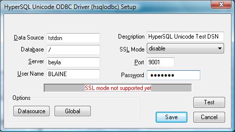 |
Then option screen 1 of 2.
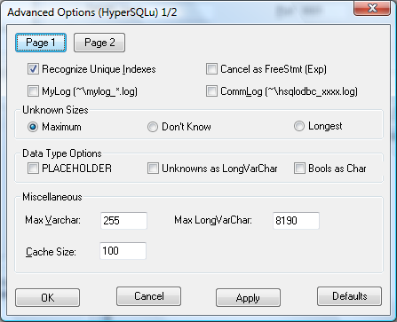 |
... and 2 of 2.
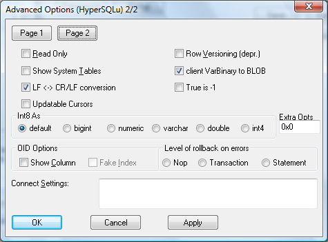 |
This section applies to both UNIX and Windows. The setting heading includes the descriptive name as shown by the Windows ODBC DS Administrator, as well as the real keyword names that UNIX users will use.
The PostgreSQL ODBC Driver product consists of two driver
variants. You should try to use the Unicode variant
first, since it supports the later and better ODBC protocol. Use the
ANSI variant if the Unicode variant won't work for
your application. The way you select the driver variant for a DSN is
platform-specific. For UNIX, set the DSN setting Driver
to the key as defined in the uniXODBC config file
/etc/unixODBC/odbcinst.ini. For UNIX, select the
driver after you click Add on the User
DSN screen, or switch it afterwards with the DSN's
Manage DSN button.
Driver settings can also be made at connection time by just appending keyword abbreviation/value assignment pairs to the ODBC connection string, delimiting each such pair with a semicolon. Base connection Strings are language-dependent, but you always append a String in this form
;A0=0;B9=1
See the Table below for a concise list of the abbreviations you may use. The appendix also shows the default values for settings (this is really only necessary for UNIX users, since the Windows DSN manager always shows the current effective value).
Runtime Driver Settings
|
Database | ODBC does not allow an empty string for a DSN database name. Therefore, you must specify DSN database name of "/" (without the quotes) to indicate the default database |
|
Recognize Unique Indexes | |
|
Cancel as FreeStmt | Find out what this experimental feature is for. |
|
MyLog | Enables fairly verbose runtime logging to the indicated file. With value 1 will write coded mylog() messages to the MyLog file. With value 2 will write both mylog() and inolog() messages to MyLog file. |
|
CommLog | Enables runtime communiction logging to the indicated file. With value 1, will write coded qlog() messages to the CommLog. |
|
Unknown Sizes |
This controls what SQLDescribeCol and SQLColAttributes will
return as to precision for the variable data
types when the precision (for example for a column) is unspecified.
For the recommended
MS Access: Seems to handle Maximum setting OK, as well as all the others. Borland: If sizes are large and lots of columns, Borland may crash badly (it doesn't seem to handle memory allocation well) if using Maximum size. |
|
Max Varchar |
Use this setting only as a work-around for client app idiocy. Generally, the database should enforce your data constraints. The maximum precision of the VARCHAR and CHAR types (perhaps others). Set to 1 larger than the value you need, to allow for null terminator characters. The default is 255 right now. 0 really means max of 0, and we need to change this ASAP so that 0 will mean unlimited. If you set this value higher than 254, Access will not let you index on varchar columns! |
|
Cache Size | When using cursors, this is the row size of the tuple cache. If not using cursors, this is how many tuples to allocate memory for at any given time. The default is 100 rows for either case. |
|
Max LongVarChar | The maximum precision of the LongVarChar type. The default is 4094 which actually means 4095 with the null terminator. You can even specify (-4) for this size, which is the odbc SQL_NO_TOTAL value. |
|
ReadOnly | Whether the datasource will allow updates. |
|
Show System Tables | The driver will treat system tables as regular tables in SQLTables. This is good for Access so you can see system tables. |
|
LF <-> CR/LF conversion | Convert Unix style line endings to DOS style. |
|
Updatable Cursors | Enable updateable cursor emulation in the driver. Fred will be implementing real Updatable ResultSets. |
|
Row Versioning | Will turn on MVCC currency control mode, once we implement this. |
|
True is -1 | Represent TRUE as -1 for compatibility with some applications. |
|
Int8 As | Define what datatype to report int8 columns as. |
|
Extra Opts |
Extra Opts: combination of the following bits.
|
|
OID Options |
|
|
OID Options |
Level of rollback on errors: Specifies what to rollback should an error occur.
default value is a sentence unit (it is a transaction unit before 8.0). |
|
Connection Settings | The driver sends these commands to the backend upon a successful connection. It sends these settings AFTER it sends the driver "Connect Settings". Use a semi-colon (;) to separate commands. This can now handle any query, even if it returns results. The results will be thrown away however! |
The HyperSQL Engine distribution contains these same ODBC client
code examples in the sample subdirectory.
See the above section for descriptions and usage details. This section just contains a list of the available settings.
Table 17.1. Settings List
| Keyword | Abbrev. | Default Val. | Purpose |
|---|---|---|---|
| Description | N/A | Data source description | |
| Servername | N/A | [required] | Name of Server |
| Port | N/A | 9001 | HyperSQL Server Listen Port |
| Username | N/A | [required] | User Name |
| Password | N/A | [required] | Password |
| Debug | B2 | 0 | MyLog logging level |
| Fetch | A7 | 100 | Fetch Max Count Test to see if this applies to EXECDIRECT and/or prepared queries |
| Socket | A8 | 4096 | Socket buffer size |
| ReadOnly | A0 | No/0 | Read Only |
| CommLog | B3 | 0 | Log communications to log file |
| UniqueIndex | N/A | 1 | Recognize unique indexes |
| UnknownSizes | A9 | 0 [= max prec. for type] | Unknown result set sizes |
| CancelAsFreeStmt | C1 | 0 | Cancel as FreeStmt |
| UnknownsAsLongVarchar | B8 | 0 | Unknowns as LongVarchar |
| BoolsAsChar | B9 | 0 | Bools as Char |
| MaxVarcharSize | B0 | 255 | Max Varchar size. Value of 0 will break everything. We will be changing 0 to mean unlimited and will then change the default to 0. |
| MaxLongVarcharSize | B1 | 8190 | Max LongVarchar size |
| RowVersioning | A4 | 0 | Row Versioning |
| ShowSystemTables | A5 | 0 | Show System Tables |
| DisallowPremature | C3 | 0 | Disallow Premature |
| UpdatableCursors | C4 | 0 | Updatable Cursors |
| LFConversion | C5 | 1 Windows, 0 UNIX | LF <-> CR/LF conversion |
| TrueIsMinus1 | C6 | 0 | True is -1 |
| BI | N/A | 0 | Datatype to report BIGINT columns as |
| LowerCaseIdentifier | C9 | 0 | Lower case identifier |
| SSLmode | CA | disable | SSL mode |
| AB | N/A | Connection string suffix options |
Abbreviations are for use in connection strings.
Table of Contents
According to the SQL Standard, the SQL Language reserved keywords cannot be used as identifiers (names of database objects such as columns and tables) without quoting.
HyperSQL has two modes of operation, which are selected with the
SET DATABASE SQL NAMES { TRUE | FALSE } to allow or
disallow the keywords as identifiers. The default mode is FALSE and allows
the use of most keywords as identifiers. Even in this mode, keywords
cannot be used as USER or ROLE identifiers. When the mode is TRUE, none of
the keywords listed below can be used as unquoted identifiers.
All keywords can be used with double quotes as identifiers. For example
CREATE TABLE "ALL" ("AND" INT, "WHEN" INT)
SELECT "AND" FROM "ALL" WHERE "WHEN" = 2022
ABS • ABSENT • ACOS • ALL • ALLOCATE • ALTER • AND • ANY
• ANY_VALUE • ARE • ARRAY • ARRAY_AGG • ARRAY_MAX_CARDINALITY • AS •
ASENSITIVE • ASIN • ASYMMETRIC • AT • ATAN • ATOMIC • AUTHORIZATION •
AVG
BEGIN • BEGIN_FRAME • BEGIN_PARTITION • BETWEEN • BIGINT
• BINARY • BIT_LENGTH • BLOB • BOOLEAN • BOTH • BY
CALL • CALLED • CARDINALITY • CASCADED • CASE • CAST •
CEIL • CEILING • CHAR • CHARACTER • CHARACTER_LENGTH • CHAR_LENGTH • CHECK
• CLOB • CLOSE • COALESCE • COLLATE • COLLECT • COLUMN • COMMIT •
COMPARABLE • CONDIITON • CONNECT • CONSTRAINT • CONTAINS • CONVERT • CORR
• CORRESPONDING • COS • COSH • COUNT • COVAR_POP • COVAR_SAMP • CREATE •
CROSS • CUBE • CUME_DIST • CURRENT • CURRENT_CATALOG • CURRENT_DATE •
CURRENT_DEFAULT_TRANSFORM_GROUP • CURRENT_PATH • CURRENT_ROLE •
CURRENT_ROW • CURRENT_SCHEMA • CURRENT_TIME • CURRENT_TIMESTAMP •
CURRENT_TRANSFORM_GROUP_FOR_TYPE • CURRENT_USER • CURSOR •
CYCLE
DATE • DAY • DEALLOCATE • DEC • DECIMAL • DECLARE •
DEFAULT • DELETE • DENSE_RANK • DEREF • DESCRIBE • DETERMINISTIC •
DISCONNECT • DISTINCT • DO • DOUBLE • DROP • DYNAMIC
EACH • ELEMENT • ELSE • ELSEIF • EMPTY • END • END_EXEC
• END_FRAME • END_PARTITION • EQUALS • ESCAPE • EVERY • EXCEPT • EXEC •
EXECUTE • EXISTS • EXIT • EXP • EXTERNAL • EXTRACT
FALSE • FETCH • FILTER • FIRST_VALUE • FLOAT • FLOOR •
FOR • FOREIGN • FRAME_ROW • FREE • FROM • FULL • FUNCTION •
FUSION
GET • GLOBAL • GRANT • GROUP • GROUPING •
GROUPS
HANDLER • HAVING • HOLD • HOUR
IDENTITY • IF • IMPORT • IN • INDICATOR • INITIAL •
INNER • INOUT • INSENSITIVE • INSERT • INT • INTEGER • INTERSECT •
INTERSECTION • INTERVAL • INTO • IS • ITERATE
JOIN • JSON • JSON_ARRAY • JSON_ARRAYAGG • JSON_EXISTS •
JSON_OBJECT • JSON_OBJECTAGG • JSON_QUERY • JSON_TABLE •
JSON_VALUE
LAG • LANGUAGE • LARGE • LAST_VALUE • LATERAL • LEAD •
LEADING • LEAST • LEAVE • LEFT • LIKE • LIKE_REGX • LISTAGG • LN • LOCAL •
LOCALTIME • LOCALTIMESTAMP • LOG • LOG10 • LOOP • LOWER • LPAD •
LTRIM
MATCH • MAX • MAX_CARDINALITY • MEMBER • MERGE • METHOD
• MIN • MINUTE • MOD • MODIFIES • MODULE • MONTH •
MULTISET
NATIONAL • NATURAL • NCHAR • NCLOB • NEW • NO • NONE •
NORMALIZE • NOT • NTH_VALUE • NTILE • NULL • NULLIF •
NUMERIC
OCCURRENCES_REGEX • OCTET_LENGTH • OF • OFFSET • OLD •
OMIT • ON • ONLY • OPEN • OR • ORDER • OUT • OUTER • OVER • OVERLAPS •
OVERLAY
PARAMETER • PARTITION • PERCENTILE_CONT •
PERCENTILE_DISC • PERCENT_RANK • PERIOD • POSITION • POSITION_REGEX •
POWER • PRECEDES • PRECISION • PREPARE • PRIMARY •
PROCEDURE
RANGE • RANK • READS • REAL • RECURSIVE • REF •
REFERENCES • REFERENCING • REGR_AVGX • REGR_AVGY • REGR_COUNT •
REGR_INTERCEPT • REGR_R2 • REGR_SLOPE • REGR_SXX • REGR_SXY • REGR_SYY •
RELEASE • REPEAT • RESIGNAL • RESULT • RETURN • RETURNS • REVOKE • RIGHT •
ROLLBACK • ROLLUP • ROW • ROWS • ROW_NUMBER • RPAD •
RTRIM
SAVEPOINT • SCOPE • SCROLL • SEARCH • SECOND • SELECT •
SENSITIVE • SESSION_USER • SET • SIGNAL • SIMILAR • SIN • SINH • SMALLINT
• SOME • SPECIFIC • SPECIFICTYPE • SQL • SQLEXCEPTION • SQLSTATE •
SQLWARNING • SQRT • STACKED • START • STATIC • STDDEV_POP • STDDEV_SAMP •
SUBMULTISET • SUBSTRING • SUBSTRING_REGEX • SUCCEEDS • SUM • SYMMETRIC •
SYSTEM • SYSTEM_TIME • SYSTEM_USER
TABLE • TABLESAMPLE • TAN • TANH • THEN • TIME •
TIMESTAMP • TIMEZONE_HOUR • TIMEZONE_MINUTE • TO • TRAILING • TRANSLATE •
TRANSLATE_REGEX • TRANSLATION • TREAT • TRIGGER • TRIM • TRIM_ARRAY • TRUE
• TRUNCATE
UESCAPE • UNDO • UNION • UNIQUE • UNKNOWN • UNNEST •
UNTIL • UPDATE • UPPER • USER • USING
VALUE • VALUES • VALUE_OF • VARBINARY • VARCHAR •
VARYING • VAR_POP • VAR_SAMP • VERSIONING
WHEN • WHENEVER • WHERE • WHILE • WIDTH_BUCKET • WINDOW
• WITH • WITHIN • WITHOUT
YEAR
When the default SET DATABASE SQL NAMES FALSE
mode is used, only a subset of SQL Standard keywords cannot be used as
HyperSQL identifiers. The keywords are as follows:
ALL • AND • ANY • ARRAY • AS • AT
BETWEEN • BOTH • BY
CALL • CASE • CAST • COALESCE • CONVERT • CORRESPONDING
• COUNT • CREATE • CROSS • CUBE
DEFAULT • DISTINCT • DO • DROP
ELSE • EVERY • EXCEPT • EXISTS
FETCH • FOR • FROM • FULL
GRANT • GROUP • GROUPING
HAVING
IN • INNER • INTERSECT • INTO • IS
JOIN
LEADING • LEFT • LIKE
MAX • MIN
NATURAL • NOT • NULLIF
ON • OR • ORDER • OUTER
PRIMARY
REFERENCES • RIGHT • ROLLUP
SELECT • SET • SOME • STDDEV_POP • STDDEV_SAMP •
SUM
TABLE • THEN • TO • TRAILING •
TRIGGER
UNION • UNIQUE • USING
VALUES • VAR_POP • VAR_SAMP
WHEN • WHERE • WITH
HyperSQL supports SQL Standard functions that are called without
parentheses. These functions include CURRENT_DATE,
LOCALTIMESTAMP, TIMEZONE_HOUR,
USER, etc. When the default SET DATABASE SQL
NAMES FALSE mode is used, keywords that are names of SQL
functions can be used as column names without double quotes in CREATE
TABLE statements . But when the identifier is a column name and is
referenced in SELECT or other statements, the keywords must be double
quoted. Otherwise the result of the SQL function is returned instead of
the column value.
HyperSQL also supports non-standard functions
SYSTIMESTAMP, CURDATE,
CURTIME, TODAY,
SYSDATE and NOW which can be called
with or without parentheses ( e.g. NOW() or
NOW ). These names can be used as column names, but the
names must be double quoted in SELECT and other statements.
Table of Contents
Database catalogs opened with the file: protocol are stored as a set of files. This document describes the contents of these files and how they are stored.
A database named 'test' is used in this description. The database files will be as follows.
Database Files
|
test.properties |
Contains the entry 'modified'. If the entry 'modified' is set to 'yes' then the database is either running or was not closed correctly. When the database is properly shutdown, 'modified' is set to 'no'. You can add the optional entry readonly=true to make the database files read only. |
|
test.script |
This file contains the SQL statements that makes up the database up to the last checkpoint. All the data for MEMORY tables is also stored in this file. |
|
test.data |
This file contains the binary data records for CACHED tables only. |
|
test.backup |
This file contains a backup of the parts of the
|
|
test.log |
This file contains the extra SQL statements that have modified the database since the last checkpoint. It is used as a redo log. |
|
test.lobs |
This file contains the lobs. If a database has no BLOB or CLOB object, this file will not be present. This file contains all the lobs that are currently in the database, as well as those that belong to rows that have been deleted since the last checkpoint. The space for deleted lobs is always reused after a CHECKPOINT. |
A CHECKPOINT is an operations that saves all the changed data and
removes the test.log followed by the creation of an
empty log. It also deletes the test.backup file. A
SHUTDOWN is equivalent to a CHECKPOINT followed by closing the
database.
The disk space needed for the database depends on the amount of
data. After the database is opened more space, up to slightly greater than
the size of the test.script and
test.data files is needed during operation.
Database is closed correctly
State after running the SHUTDOWN
statement
-
The
test.datafile is fully updated. -
There is no
test.backupfile. -
The
test.scriptcontains all the metadata and CREATE TABLE and other DDL statements. It also contains the data for MEMORY tables. -
The
test.propertiescontains the entry 'modified' set to 'no'. -
There is no
test.logfile.
Database is closed correctly with SHUTDOWN SCRIPT
State after running the SHUTDOWN SCRIPT
statement
-
The
test.datafile does not exist; all CACHED table data is now in thetest.scriptfile -
There is no
test.backupfile. -
The
test.scriptcontains all the metadata and DDL statements, followed by the data for MEMORY, CACHED and TEXT tables. -
The
test.propertiescontains the entry 'modified' set to 'no'. -
There is no
test.logfile.
Database is aborted
If the database process was terminated without a SHUTDOWN, or the SHUTDOWN IMMEDIATELY command was used, the database is in aborted state.
Aborted database state
-
The
test.propertiescontains 'modified=yes'. -
The
test.scriptcontains a snapshot of the database at the last checkpoint. -
The
test.datafile is not necessarily consistent. -
The
test.backupfile contains just sections of the originaltest.datafile that correspond totest.scriptat the time of the last checkpoint. -
The
test.logfile contain all data change statements executed since the last checkpoint. As a result of abnormal termination, the end of file may be incomplete.
The database engine performs the following procedures internally in different circumstances.
Procedure B.1. Clean HyperSQL database shutdown
-
The
test.datafile is written completely (all the modified cached table rows are written out) and closed. -
The file
test.script.newis created using the current state of the database. -
The entry 'modified' in the properties file is set to 'yes-new-files' (Note: after this step, the
test.dataandtest.script.newfiles constitute the database) -
The file
test.logis deleted -
The file
test.scriptis deleted -
The file
test.script.newis renamed totest.script -
The file
test.backupis deleted -
The entry 'modified' in the properties file is set to 'no'
Procedure B.2. Opening the Database
-
Check if the database files are in use by checking a special
test.lckfile. -
See if the
test.propertiesfile exists, otherwise create it. -
If the
test.scriptdid not exist, then this is a new database. -
If it is an existing database, check in the
test.propertiesfile if 'modified=yes'. In this case the RESTORE operation is performed before the database is opened normally. -
Otherwise, if in the
test.propertiesfile 'modified=yes-new-files', then the (old)test.backupandtest.scriptfiles are deleted if they exist and the newtest.script.newfile is renamed totest.script. -
Open the
test.scriptfile and create the database objects. -
Create the empty
test.logto append any data change statements.
The current test.data file is not necessarily
consistent. The database engine takes these steps:
Procedure B.3. Restore a Database
-
Restore the old
test.datafile from the backup by copying the original sections from thetest.backupfile. -
Execute all the statements in the
test.scriptfile. -
Execute all statements in the
test.logfile. If due to incomplete statements in this file an exception is thrown, the rest of the lines in thetest.logfile are ignored. This can be overridden with the database connection propertyhsqldb.full_log_replay=truewhich results in the startup process to fail and allows the user to examine and edit thetest.logfile. -
Close the database files.
-
Open the restored database.
Table of Contents
The hsqldb.jar file supplied in the lib
directory of the zip release package is built and tested with Java 11. An
separate jar for Java 8 is also supplied in the same directory. The jars
have been tested extensively with the latest Java versions. You can also
find the official jars in major maven repositories as well as downloads
from hsqldb.org.
The Gradle task / Ant target explainjars
reports the versions of Java and Ant actually used.
If you want to change Ant or Gradle build settings, edit the text
file build.properties in the HyperSQL
build directory (creating it if it doesn't exist
yet), and enter your properties using Java properties file syntax. (You
can also use local-docbook.properties in the same way
for DocBook-specific properties).
Unlike most software build systems, you do not need to have the
Gradle system installed on your computer to use it. You don't need to
understand the details to use it, but this is the purpose of the
gradlew wrapper scripts that you
can see in HyperSQL's build directory. If you want or
need to learn more about Gradle, you can start on the Gradle web site.
| Gradle honors JAVA_HOME |
|---|---|
|
Gradle can find the Java to use by finding out where
|
| Rare Gotcha |
|---|---|
|
Depending on your operating system, version, and how you
installed your JDK, Gradle may not be able to find the JDK. Gradle will
inform you if this happens. The easiest way to fix this problem is to
set environmental variable |
You can invoke Gradle builds from the command-line.
-
Get a command-line shell. Windows users can use either or , and enter "
cmd". Non-windows users will know how to get a shell. -
In the shell, cd to the
builddirectory under the root directory where you extracted or installed HyperSQL to. (Operating system search or find functions can be used if you can't find it quickly by poking around on the command line or with Windows Explorer, etc.). -
Windows users can ignore this step. UNIX shell users should ensure that the current directory (
.) is in their search path, or prefix theirgradlewcommand in the next step with./(e.g., like./gradlew). -
In the shell, run
gradlewfor a build.If you ran just
gradlew, then you will be presented with simple instructions for how to do everything that you want to do. Basically, you will run the samegradlewcommand repeatedly, with different switches and arguments for each build target.Note Gradle's -v switch reports version details more directly than the
explainjarstask does, from the operating system version to the Groovy version (the language interpreter used for Gradle instructions).
For example, the command below builds the
hsqldb.jar file:
gradlew hsqldb
The Gradle invocations actually run Ant build targets. Some of the targets are listed in the next section.
You should use version 1.9 or 1.10 of Ant (Another Neat Tool) to do Ant builds with HyperSQL.
Ant is a part of the Apache Project.
- Home of the Apache Ant project
- The Installing Ant page of the Ant Manual. Follow the directions for your platform.
Once you have unpacked the zip package for hsqldb, under the
/hsqldb folder, in /build
there is a build.xml file that builds the
hsqldb.jar with Ant (Ant must be already
installed). To use it, change to /build then
type:
ant -projecthelp
This displays the available Ant targets, which you can supply as command line arguments to ant. These include
|
hsqldb | to build the hsqldb.jar file. This
contains the engine and the GUI database manager. |
|
explainjars | Lists all targets which build jar files, with an explanation of the purposes of the different jars. |
|
clean | to clean up the /classes directory that is created during a build. |
|
clean-all | to remove the old jar and doc files as well as clean. |
|
javadoc | to build javadoc for all public classes accessible to user applications. |
|
dbmanswing | to build the dbmanagerswing.jar
file |
|
hsqldbmain | to build a smaller jar for HSQLDB that does not contain utilities |
|
hsqldbmin | to build a small jar that supports in-process catalogs, but not running HyperSQL Servers. |
|
sqltool | to build sqltool.jar, which contains only the SqlTool classes. |
|
... | Many more targets are available. Run ant
-p and ant explainjars. |
HSQLDB can be built in any combination of JRE (Java Runtime Environment) versions and many jar file sizes.
A jar built with an older JRE is compatible for use with a newer JRE. You can compile with Java 8 and run with 11 but the Java module capabilities of HyperSQL will be not be available.
The smallest engine jar (hsqldbmin.jar)
contains the engine and the HSQLDB JDBC Driver client. The default size
(hsqldb.jar) also contains server mode support and
the utilities. The largest size
(hsqldbtest.jar)includes some test classes as well.
Before building the hsqldbtest.jar package, you
should download the junit jar from http://www.junit.org and put it in the
/lib directory, alongside
servlet.jar, which is included in the .zip
package.
If you want your code built for high performance, as opposed to
debugging (in the same way that we make our production distributions),
make a file named build.properties in your build
directory with the contents
build.debug: false
The resulting Java binaries will be faster and smaller, at the cost of exception stack traces not identifying source code locations (which can be extremely useful for debugging).
After installing Ant on your system use the following command
from the /build directory. Just run ant
explainjars for a concise list of all available jar
files.
ant explainjars
The command displays a list of different options for building different sizes of the HSQLDB Jar. The default is built using:
The Ant method always builds a jar with the JDK that is used by Ant and specified in its JAVA_HOME environment variable.
The jars can be compiled with JDK 8 or later. Build has been tested under JDK versions 8, 11, and 21. The same Ant version can be used with all the tested JDKs.
The Ant build.xml can be used with most IDEs to build the Jar targets. All HyperSQL source files are supplied ready to compile. It is therefore possible to compile the sources without using Ant directly.
CodeSwitcher is a tool to manage conditional compilation of Java source code. It is something like a precompiler in C but it works directly on the source code and does not create intermediate output or extra files.
CodeSwitcher reads the source code of a file, removes comments where appropriate and comments out the blocks that are not used for a particular version of the file. This operation is done for all files of a defined directory, and all subdirectories. The current version of HSQLDB does not use the CodeSwitcher.
Example C.2. Example source code before CodeSwitcher is run
...
//#ifdef JAVA8
properties.store(out,"hsqldb database");
//#else
/*
properties.save(out,"hsqldb database");
*/
//#endif
...
The next step is to run CodeSwitcher.
The '.' means the program works on the current directory (all
subdirectories are processed recursively). -JAVA8 means
the code labelled with JAVA8 must be switched off.
Example C.4. Source code after CodeSwitcher processing
...
//#ifdef JAVA8
/*
pProperties.store(out,"hsqldb database");
*/
//#else
pProperties.save(out,"hsqldb database");
//#endif
...
For detailed information on the command line options run
java org.hsqldb.util.CodeSwitcher. Usage examples
can be found in the build.xml file in the /build
directory.
Java 11 is the only supported JDK for building the documentation.
The JavaDoc can be built simply by invoking the javadoc task/target with Gradle or Ant.
The two Guides (the one you are reading now plus the Utilities user
guide) are in DocBook XML source format. To rebuild to PDF or one of the
HTML output formats from the XML source, run the Gradle target
gen-docs (or the Ant target
gen-docs). Instructions will be displayed. In
particular
- Obtain the HyperSQL documentation source. We no longer include our Guide source files in our main distribution zip file, in order to keep it small. You may want to build from the trunk branch or the latest release tag. You can download a static snapshot tarball from https://sourceforge.net/p/hsqldb/svn/HEAD/tree/ or you can use a Subversion client such as TortoiseSVN to export a snapshot or check out a work area.
- You must locally install the DocBook set of image files,
which are available for download from Sourceforge. The
gen-docstask/target will tell you of a Gradle task that you can use to download and install them automatically. This Gradle task,installDbImages, will tell you how to edit a properties text file to tell it what directory to install the files into. (Command-line, as opposed to GUI, builders, can use the Gradle-Pswitch to set the property, instead of editing, if they prefer). - You can optionally install the entire DocBook style sheets
(instead of just the DocBook images within it), character entity
definitions, and RNG schema file, to speed up doc build times and
minimize dependency of future builds upon network or Internet. An
intermediate approach would be to install these resources onto an
HTTP server or shared network drive of your own. See the comments at
the top of the file
build.xmlin the HyperSQLbuilddirectory about where to obtain these things and how to hook them in. The same Gradle taskinstallDbImagesexplained above can download and install the entire style sheet bundle (this option is offered the first time that you run theinstallDbImagestask).
![[Tip]](../images/db/tip.png) | Tip |
|---|---|
|
If running Gradle, you probably want to turn logging up to level info for generation and validation tasks, because the default warn/lifecycle level doesn't give much feedback. |
The task/target validate-docs is also very
useful to DocBook builders.
The documentation license does not allow you to post
modifications to our guides, but you can modify them for internal use by
your organization, and you can use our DocBook system to write new DocBook
documents related or unrelated to HyperSQL. To create new DocBook
documents, create a subdirectory off of doc-src for
each new document, with the main DocBook source file within having same
name as the directory plus .xml. See the peer directory
util-guide or guide as an
example. If you use the high-level tasks/target
gen-docs or validate-docs, then copy
and paste to add new stanzas to these targets in file
build.xml.
Editors of DocBook documents (see previous paragraph for motive)
may find it useful to have a standalone XML validator so you can do your
primary editing without involvement of the build system. Use the Gradle
target standaloneValidation for this. It will tell you
how to set a build property to tell it where to install the validator, and
will give instructions on how to use it.
There are several properties that can be used to dramatically reduce
run times for partial doc builds. Read about these properties in comment
at the top of the file build-docbook.xml in the
build directory.
- validation.skip
- html.skip
- chunk.skip
- fo.skip
- pdf.skip
- doc.name
- doc.target
See the file doc-src/readme-docauthors.txt
for details about our DocBook build system.
Table of Contents
OpenOffice.org / LibreOffice / ApacheOpenOffice includes HyperSQL and uses it for embedded databases. Our collaboration with OpenOffice.org developers over 6 years has benefited the development and maturity of HyperSQL. Before integration into OOo, HyperSQL was intended solely for application-specific database access. The application developer was expected to resolve any integration issues. Because OpenOffice.org is used by a vast range of users, from schoolchildren to corporate developers, a much higher level of quality assurance has been required. We have achieved it with constant help and feedback from OOo users and developers.
Apart from embedded use, you may want to use OpenOffice / LibreOffice with a HyperSQL server instance. The typical use for this is to allow multiple office users access to the same database.
There is also a strong case for using OpenOffice to develop your database schema and application, even if the database is intended for your own application, rather than OpenOffice.
HyperSQ version 1.8.0 is included in OOo, ApacheOpenOffice and LibreOffice. You can simply replace the jar with a HyperSQL version 2.7 jar to use the latest capabilities with external databases. It is not yet possible to create and use embedded databases with this version.
HyperSQL version 2.x jar will hopefully be included in the future versions of ApacheOpenOffice and LibreOffice.
OpenOffice is a powerful database front end. If you want to create schemas, edit tables, edit the database contents manually, design and produce well-formatted reports, then OpenOffice is probably the best open source tools currently available.
To connect from OpenOffice to your database, first run a local server instance for the database. This is describes in the Network Listeners chapter of this guide.
When you connect from OpenOffice.org, you must specify connection to an external database and use the URL property "default_schema=true". For example, the URL to connect the local database may be like
jdbc;hsqldb:hsql://localhost/mydb;default_schema=true
The only current limitation is that OpenOffice only works with the PUBLIC schema. This limitation will hopefully disappear in the future versions of OOo.
There will hopefully be a HyperSQL 2.x jar in future versions of OpenOffice.
You may already have an OOo database file, which you want to use outside OOo, or as a server database. The file is in fact in the standard ZIP format and contains the normal HyperSQL database files. Just use a utility such as 7Zip to expand the .odb file. In the /db directory, there are files such as .script, .data, etc. Just rename these files into mydb.script, mydb.data, etc. You can now open the mydb database directly with HyperSQL as an embedded database or as a server instance.
Since 2021, two new OOo and LO extensions are developed and maintained on GitHub by the developer prrvchr. These extensions make it easy to use the latest version of HSQLDB 2.x with the latest versions of the Base program. One extension simply adds and loads the HSQLDB 2.x jar, ready for use. It also allows updating the jar to the latest version. The second extension extracts the database from the .odb file in the same directory and connects to the extracted database files.
The simple driver: https://prrvchr.github.io/jdbcDriverOOo/
The driver that extracts the files: https://prrvchr.github.io/HyperSQLOOo/
The extensions are easy to use, with clear visual instructions on how to add the extensions to the Office suite and how to create and open databases.
HyperSQL files referred to in the text may be retrieved from the canonical HyperSQL documentation site, http://hsqldb.org/doc/2.0, or from the same location you are reading this page from.
| Note |
|---|---|
|
If you are reading this document with a standalone PDF reader, only the http://hsqldb.org/doc/2.0/... links will function. |
Pairs of local + http://hsqldb.org/doc/2.0 links for referenced files.
-
Local: ../apidocs/org.hsqldb/org/hsqldb/jdbc/JDBCConnection.html
http://hsqldb.org/doc/2.0/apidocs/org.hsqldb/org/hsqldb/jdbc/JDBCConnection.html
-
Local: ../apidocs/org.hsqldb/org/hsqldb/jdbc/JDBCDriver.html
http://hsqldb.org/doc/2.0/apidocs/org.hsqldb/org/hsqldb/jdbc/JDBCDriver.html
-
Local: ../apidocs/org.hsqldb/org/hsqldb/jdbc/JDBCDatabaseMetaData.html
http://hsqldb.org/doc/2.0/apidocs/org.hsqldb/org/hsqldb/jdbc/JDBCDatabaseMetaData.html
-
Local: ../apidocs/org.hsqldb/org/hsqldb/jdbc/JDBCResultSet.html
http://hsqldb.org/doc/2.0/apidocs/org.hsqldb/org/hsqldb/jdbc/JDBCResultSet.html
-
Local: ../apidocs/org.hsqldb/org/hsqldb/jdbc/JDBCStatement.html
http://hsqldb.org/doc/2.0/apidocs/org.hsqldb/org/hsqldb/jdbc/JDBCStatement.html
-
Local: ../apidocs/org.hsqldb/org/hsqldb/jdbc/JDBCPreparedStatement.html
http://hsqldb.org/doc/2.0/apidocs/org.hsqldb/org/hsqldb/jdbc/JDBCPreparedStatement.html
-
Local: ../apidocs/org.hsqldb/org/hsqldb/util/MainInvoker.html
http://hsqldb.org/doc/2.0/apidocs/org.hsqldb/org/hsqldb/util/MainInvoker.html
-
Local: ../apidocs/index.html
-
Local: ../verbatim/src/org/hsqldb/server/Servlet.java
http://hsqldb.org/doc/2.0/verbatim/src/org/hsqldb/server/Servlet.java
-
Local: ../verbatim/src/org/hsqldb/Tokens.java
http://hsqldb.org/doc/2.0/verbatim/src/org/hsqldb/Tokens.java
-
Local: ../verbatim/src/org/hsqldb/server/WebServer.java
http://hsqldb.org/doc/2.0/verbatim/src/org/hsqldb/server/WebServer.java
-
Local: ../verbatim/src/org/hsqldb/test/TestBase.java
http://hsqldb.org/doc/2.0/verbatim/src/org/hsqldb/test/TestBase.java
-
Local: ../verbatim/src/org/hsqldb/trigger/Trigger.java
http://hsqldb.org/doc/2.0/verbatim/src/org/hsqldb/trigger/Trigger.java
-
Local: ../verbatim/src/org/hsqldb/sample/TriggerSample.java
http://hsqldb.org/doc/2.0/verbatim/src/org/hsqldb/test/sample/TriggerSample.java
-
Local: ../verbatim/src/org/hsqldb/util/MainInvoker.java
http://hsqldb.org/doc/2.0/verbatim/src/org/hsqldb/util/MainInvoker.java
-
Local: ../verbatim/sample/acl.txt
Symbols
- _SYSTEM Role, Built-In Roles and Users
A
- ABS function, Numeric Functions
- Access Rights, Access Rights
- ACOS function, Numeric Functions
- ACTION_ID function, System Functions
- ADD_MONTHS function, Functions for Datetime Arithmetic
- ADD COLUMN, Table Manipulation
- add column identity generator or sequence, Table Manipulation
- ADD CONSTRAINT, Table Manipulation
- ADD DOMAIN CONSTRAINT, Domain Creation and Manipulation
- ADD SYSTEM PERIOD, Table Manipulation
- ADD SYSTEM VERSIONING, Table Manipulation
- ADMINISTRABLE_ROLE_AUTHORIZATIONS, SQL Standard Views
- Admin USER, Built-In Roles and Users
- aggregate function, Aggregate Functions
- ALL and ANY predicates, Predicates
- ALTER COLUMN, Table Manipulation
- alter column identity generator, Table Manipulation
- alter column nullability, Table Manipulation
- ALTER CONSTRAINT, Other Schema Objects Creation and Alteration
- ALTER DOMAIN, Domain Creation and Manipulation
- ALTER INDEX, Other Schema Objects Creation and Alteration
- ALTER routine, Routine Creation
- ALTER SEQUENCE, Sequence Creation
- ALTER SESSION, Session and Transaction Control Statements
- ALTER TABLE, Table Manipulation
- ALTER USER ... SET INITIAL SCHEMA, Statements for Authorization and Access Control
- ALTER USER ... SET LOCAL, Statements for Authorization and Access Control
- ALTER USER ... SET PASSWORD, Statements for Authorization and Access Control
- ALTER view, View Creation and Manipulation
- APPLICABLE_ROLES, SQL Standard Views
- ASCII function, String and Binary String Functions
- ASCIISTR function, String and Binary String Functions
- ASIN function, Numeric Functions
- ASSERTIONS, SQL Standard Views
- as subquery clause in table definition, Table Creation
- ATAN2 function, Numeric Functions
- ATAN function, Numeric Functions
- Authorisation and Access Control, Authorizations and Access Control
- AUTHORIZATION IDENTIFIER, Authorizations and Access Control
- AUTHORIZATIONS, SQL Standard Views
B
- BACKUP DATABASE, System Operations
- BETWEEN predicate, Predicates
- binary literal, Literals
- BINARY types, Binary String Types
- BIT_LENGTH function, String and Binary String Functions
- BITAND function, Numeric Functions
- BITANDNOT function, Numeric Functions
- bit literal, Literals
- BITNOT function, Numeric Functions
- BITOR function, Numeric Functions
- BIT types, Bit String Types
- BITXOR function, Numeric Functions
- boolean literal, Literals
- BOOLEAN types, Boolean Type
- boolean value expression, Value Expression
- Built-in Roles and Users, Built-In Roles and Users
C
- CARDINALITY function, Array Functions
- CASCADE or RESTRICT, Common Elements and Statements
- case expression, Value Expression
- CASEWHEN function, General Functions
- CASE WHEN in routines, Conditional Statements
- CAST, Value Expression
- CEIL function, Numeric Functions
- CHANGE_AUTHORIZATION, Built-In Roles and Users
- CHAR_LENGTH, String and Binary String Functions
- CHARACTER_LENGTH, String and Binary String Functions
- CHARACTER_SETS, SQL Standard Views
- character literal, Literals
- CHARACTER types, Character String Types
- character value function, Value Expression
- CHAR function, String and Binary String Functions
- CHECK_CONSTRAINT_ROUTINE_USAGE, SQL Standard Views
- CHECK_CONSTRAINTS, SQL Standard Views
- CHECK constraint, Table Creation
- CHECKPOINT, System Operations
- COALESCE expression, Value Expression
- COALESCE function, General Functions
- COLLATE, Other Syntax Elements
- COLLATIONS, SQL Standard Views
- COLUMN_COLUMN_USAGE, SQL Standard Views
- COLUMN_DOMAIN_USAGE, SQL Standard Views
- COLUMN_PRIVILEGES, SQL Standard Views
- COLUMN_UDT_USAGE, SQL Standard Views
- column DEFAULT clause, Table Creation
- column definition, Table Creation
- column name list, Column Name List
- column reference, References, etc.
- COLUMNS, SQL Standard Views
- COMMENT, Commenting Objects
- COMMIT, Session and Transaction Control Statements
- comparison predicate, Predicates
- CONCAT_WS function, String and Binary String Functions
- CONCAT function, String and Binary String Functions
- CONSTRAINT, Other Syntax Elements
- CONSTRAINT_COLUMN_USAGE, SQL Standard Views
- CONSTRAINT_PERIOD_USAGE, SQL Standard Views
- CONSTRAINT_TABLE_USAGE, SQL Standard Views
- CONSTRAINT (table constraint), Table Creation
- CONSTRAINT name and characteristics, Table Creation
- CONTAINS predicate, Predicates
- contextually typed value specification, References, etc.
- CONVERT function, General Functions
- COS function, Numeric Functions
- COSH function, Numeric Functions
- COT function, Numeric Functions
- CREATE_SCHEMA Role, Built-In Roles and Users
- CREATE AGGREGATE FUNCTION, Definition of Aggregate Functions
- CREATE ASSERTION, Other Schema Objects Creation and Alteration
- CREATE CAST, Other Schema Objects Creation and Alteration
- CREATE CHARACTER SET, Other Schema Objects Creation and Alteration
- CREATE COLLATION, Other Schema Objects Creation and Alteration
- CREATE DOMAIN, Domain Creation and Manipulation
- CREATE FUNCTION, Routine Definition
- CREATE INDEX, Other Schema Objects Creation and Alteration
- CREATE PROCEDURE, Routine Definition
- CREATE ROLE, Statements for Authorization and Access Control
- CREATE SCHEMA, Schema Creation
- CREATE SEQUENCE, Sequence Creation
- CREATE SYNONYM, Other Schema Objects Creation and Alteration
- CREATE TABLE, Table Creation
- CREATE TRANSLATION, Other Schema Objects Creation and Alteration
- CREATE TRIGGER, Trigger Creation, Trigger Creation
- CREATE TYPE, Other Schema Objects Creation and Alteration
- CREATE USER, Statements for Authorization and Access Control
- CREATE VIEW, View Creation and Manipulation
- CROSS JOIN, Joined Table
- CRYPT_KEY function, System Functions
- CURDATE function, Functions to Report the Current Datetime
- CURRENT_CATALOG function, System Functions
- CURRENT_DATE function, Functions to Report the Current Datetime
- CURRENT_ROLE function, System Functions
- CURRENT_SCHEMA function, System Functions
- CURRENT_TIME function, Functions to Report the Current Datetime
- CURRENT_TIMESTAMP function, Functions to Report the Current Datetime
- CURRENT_USER function, System Functions
- CURRENT VALUE FOR, Value Expression
- CURTIME function, Functions to Report the Current Datetime
D
- DATA_TYPE_PRIVILEGES, SQL Standard Views
- DATABASE_ISOLATION_LEVEL function, System Functions
- DATABASE_NAME function, System Functions
- DATABASE_TIMEZONE function, Functions to Report the Time Zone.
- DATABASE_VERSION function, System Functions
- DATABASE function, System Functions
- DATE_ADD function, Functions for Datetime Arithmetic
- DATE_SUB function, Functions for Datetime Arithmetic
- DATEADD function, Functions for Datetime Arithmetic
- DATEDIFF function, Functions for Datetime Arithmetic
- DATENAME, DATEPART and EOMONTH functions, Functions to Extract an Element of a Datetime
- datetime and interval literal, Literals
- Datetime Operations, Datetime types
- DATETIME types, Datetime types
- datetime value expression, Value Expression
- datetime value function, Value Expression
- DAYNAME function, Functions to Extract an Element of a Datetime
- DAYOFMONTH function, Functions to Extract an Element of a Datetime
- DAYOFWEEK function, Functions to Extract an Element of a Datetime
- DAYOFYEAR function, Functions to Extract an Element of a Datetime
- DAYS function datetime, Functions to Extract an Element of a Datetime
- DBA Role, Built-In Roles and Users
- DECLARE CURSOR, Cursor Declaration
- DECLARE HANDLER, Handlers
- DECLARE variable, Variables
- DECODE function, General Functions
- DEGREES function, Numeric Functions
- DELETE FROM, Delete Statement
- Derived Table, Derived Table
- DETERMINISTIC characteristic, Routine Characteristics
- DIAGNOSTICS function, System Functions
- DIFFERENCE function, String and Binary String Functions
- DISCONNECT, Session and Transaction Control Statements
- DISTINCT, Grouping Operations
- DOMAIN_CONSTRAINTS, SQL Standard Views
- DOMAINS, SQL Standard Views
- DROP ASSERTION, Other Schema Objects Creation and Alteration
- DROP CAST, Other Schema Objects Creation and Alteration
- DROP CHARACTER SET, Other Schema Objects Creation and Alteration
- DROP COLLATION, Other Schema Objects Creation and Alteration
- DROP COLUMN, Table Manipulation
- drop column identity generator, Table Manipulation
- DROP CONSTRAINT, Table Manipulation
- DROP DEFAULT (table), Table Manipulation
- DROP DOMAIN, Domain Creation and Manipulation
- DROP DOMAIN CONSTRAINT, Domain Creation and Manipulation
- DROP DOMAIN DEFAULT, Domain Creation and Manipulation
- DROP INDEX, Other Schema Objects Creation and Alteration
- DROP ROLE, Statements for Authorization and Access Control
- DROP routine, Routine Creation
- DROP SCHEMA, Schema Creation
- DROP SEQUENCE, Sequence Creation
- DROP SYNONYM, Other Schema Objects Creation and Alteration
- DROP SYSTEM PERIOD, Table Manipulation
- DROP SYSTEM VERSIONING, Table Manipulation
- DROP TABLE, Table Creation
- DROP TRANSLATION, Other Schema Objects Creation and Alteration
- DROP TRIGGER, Trigger Creation, Trigger Creation
- DROP USER, Statements for Authorization and Access Control
- DROP VIEW, View Creation and Manipulation
- DYNAMIC RESULT SETS, Routine Characteristics
E
- ELEMENT_TYPES, SQL Standard Views
- ENABLED_ROLES, SQL Standard Views
- EQUALS predicate, Predicates
- EXISTS predicate, Predicates
- EXP function, Numeric Functions
- EXPLAIN PLAN, Indexes Used in SELECT and DML Statements
- EXPLAIN REFERENCES, References to Database Objects
- expression, Value Expression
- external authentication, Authentication Control
- EXTERNAL NAME, Routine Definition
- EXTRACT function, Functions to Extract an Element of a Datetime
F
- Fine Grained Data Access Control, Fine-Grained Data Access Control
- FLOOR function, Numeric Functions
- FOREIGN KEY constraint, Table Creation
- FOR loop in routines, Iterated FOR Statement
- FROM_BASE64 function, String and Binary String Functions
- FROM_TZ function, Functions to Convert or Format a Datetime
G
- generated column specification, Table Creation
- GET DIAGNOSTICS, Diagnostics and State
- GRANTED BY, Statements for Authorization and Access Control
- GRANT privileges, Statements for Authorization and Access Control
- GRANT role, Statements for Authorization and Access Control
- GREATEST function, General Functions
- GROUP BY, Grouping Operations
- GROUPING OPERATIONS, Grouping Operations
H
- HAVING, Grouping Operations
- HEX function, String and Binary String Functions
- HEXTORAW function, String and Binary String Functions
- HOUR function, Functions to Extract an Element of a Datetime
I
- identifier chain, References, etc.
- identifier definition, Common Elements and Statements
- IDENTITY function, System Functions
- IF EXISTS, Common Elements and Statements
- IF NOT EXISTS, Common Elements and Statements
- IFNULL function, General Functions
- IF STATEMENT, Conditional Statements
- INFORMATION_SCHEMA_CATALOG_NAME, SQL Standard Views
- IN predicate, Predicates
- INSERT function, String and Binary String Functions
- INSERT INTO, Insert Statement
- INSTR function, String and Binary String Functions
- interval absolute value function, Value Expression
- interval term, Value Expression
- INTERVAL types, Interval Types
- IS_AUTOCOMMIT function, System Functions
- IS_READONLY_DATABASE_FILES function, System Functions
- IS_READONLY_DATABASE function, System Functions
- IS_READONLY_SESSION function, System Functions
- IS DISTINCT predicate, Predicates
- ISNULL function, General Functions
- IS NULL predicate, Predicates
- ISOLATION_LEVEL function, System Functions
J
- JOIN USING, Joined Table
- JOIN with condition, Joined Table
- JSON_ARRAY_AGG function, JSON Functions
- JSON_ARRAY function, JSON Functions
- JSON_OBJECT function, JSON Functions
K
- KEY_COLUMN_USAGE, SQL Standard Views
- KEY_PERIOD_USAGE, SQL Standard Views
L
- LANGUAGE, Routine Characteristics
- LAST_DAY function, Functions for Datetime Arithmetic
- LATERAL derived table, Lateral
- LCASE function, String and Binary String Functions
- LEAST function, General Functions
- LEFT function, String and Binary String Functions
- LENGTH function, String and Binary String Functions
- like clause in table definition, Table Creation
- LIKE predicate, Predicates
- Listing Users and Roles, Listing Users and Roles
- LN function, Numeric Functions
- LOAD_FILE function, General Functions
- LOB_ID function, System Functions
- LOCALTIME function, Functions to Report the Current Datetime
- LOCALTIMESTAMP function, Functions to Report the Current Datetime
- LOCATE function, String and Binary String Functions
- LOCK TABLE, Session and Transaction Control Statements
- LOG10 function, Numeric Functions
- LOG function, Numeric Functions
- LOOP in routines, Iterated Statements
- LOWER function, String and Binary String Functions
- LPAD function, String and Binary String Functions
- LTRIM function, String and Binary String Functions
M
- MATCH predicate, Predicates
- MAX_CARDINALITY function, Array Functions
- MERGE INTO, Merge Statement
- MINUTE function, Functions to Extract an Element of a Datetime
- MOD function, Numeric Functions
- MONTH function, Functions to Extract an Element of a Datetime
- MONTHNAME function, Functions to Extract an Element of a Datetime
- MONTHS_BETWEEN function, Functions for Datetime Arithmetic
N
- name resolution, Naming
- naming in joined table, Naming
- naming in select list, Naming
- NATURAL JOIN, Joined Table
- NAVL function, Numeric Functions
- NEXT_DAY function, Functions for Datetime Arithmetic
- NEXT VALUE FOR, Value Expression
- NOW function, Functions to Report the Current Datetime
- NULLIF function, General Functions
- NULL INPUT, Routine Characteristics
- numeric literal, Literals
- NUMERIC types, Numeric Types
- numeric value expression, Value Expression
- numeric value function, Value Expression
- NUMTODSINTERVAL function, Functions to Convert or Format a Datetime
- NUMTOYMINTERVAL function, Functions to Convert or Format a Datetime
- NVL2 function, General Functions
- NVL function, General Functions
O
- OCTET_LENGTH function, String and Binary String Functions
- ON UPDATE clause (table constraint), Table Creation
- OTHER type, Storage and Handling of Java Objects
- OUTER JOIN, Joined Table
- OVERLAPS predicate, Predicates
- OVERLAY function, String and Binary String Functions
P
- PARAMETERS, SQL Standard Views
- password complexity, Authentication Control
- PATH, Other Syntax Elements
- PERFORM CHECK INDEX, Data Management Statements
- PERFORM EXPORT DSV, Data Management Statements
- PERFORM EXPORT SCRIPT, Data Management Statements
- PERFORM IMPORT DSV file, Data Management Statements
- PERFORM IMPORT SCRIPT, Data Management Statements
- PERIODS, SQL Standard Views
- PI function, Numeric Functions
- POSITION_ARRAY function, Array Functions
- POSITION function, String and Binary String Functions
- POWER function, Numeric Functions
- PRECEDES predicate, Predicates
- PRIMARY KEY constraint, Table Creation
- PUBLIC Role, Built-In Roles and Users
Q
- QUARTER function, Functions to Extract an Element of a Datetime
- query specification, Query Specification
R
- RADIANS function, Numeric Functions
- RAND function, Numeric Functions
- RAWTOHEX function, String and Binary String Functions
- REFERENTIAL_CONSTRAINTS, SQL Standard Views
- REGEXP_COUNT function, String and Binary String Functions
- REGEXP_INSTR function, String and Binary String Functions
- REGEXP_LIKE function, String and Binary String Functions
- REGEXP_MATCHES function, String and Binary String Functions
- REGEXP_REPLACE function, String and Binary String Functions
- REGEXP_SUBSTR function, String and Binary String Functions
- REGEXP_SUBSTRING_ARRAY function, String and Binary String Functions
- REGEXP_SUBSTRING function, String and Binary String Functions
- RELEASE SAVEPOINT, Session and Transaction Control Statements
- RENAME, Renaming Objects
- REPEAT ... UNTIL loop in routines, Iterated Statements
- REPEAT function, String and Binary String Functions
- REPLACE function, String and Binary String Functions
- replicated databases, Replicated Databases
- Reserved Keywords, List of SQL Standard Keywords
- RESIGNAL STATEMENT, Raising Exceptions
- RETURN, Return Statement
- RETURNS, Routine Definition
- REVERSE function, String and Binary String Functions
- REVOKE privileges, Statements for Authorization and Access Control
- REVOKE ROLE, Statements for Authorization and Access Control
- RIGHT function, String and Binary String Functions
- ROLE_AUTHORIZATION_DESCRIPTORS, SQL Standard Views
- ROLE_COLUMN_GRANTS, SQL Standard Views
- ROLE_ROUTINE_GRANTS, SQL Standard Views
- ROLE_TABLE_GRANTS, SQL Standard Views
- ROLE_UDT_GRANTS, SQL Standard Views
- ROLE_USAGE_GRANTS, SQL Standard Views
- ROLLBACK, Session and Transaction Control Statements
- ROLLBACK TO SAVEPOINT, Session and Transaction Control Statements
- ROUND function datetime, Functions for Datetime Arithmetic
- ROUND number function, Numeric Functions
- ROUTINE_COLUMN_USAGE, SQL Standard Views
- ROUTINE_JAR_USAGE, SQL Standard Views
- ROUTINE_PERIOD_USAGE, SQL Standard Views
- ROUTINE_PRIVILEGES, SQL Standard Views
- ROUTINE_ROUTINE_USAGE, SQL Standard Views
- ROUTINE_SEQUENCE_USAGE, SQL Standard Views
- ROUTINE_TABLE_USAGE, SQL Standard Views
- routine body, Routine Definition
- routine invocation, Other Syntax Elements
- ROUTINES, SQL Standard Views
- ROW_NUMBER function, System Functions
- ROWNUM function, System Functions
- row value expression, Value Expression
- RPAD function, String and Binary String Functions
- RTRIM function, String and Binary String Functions
S
- SAVEPOINT, Session and Transaction Control Statements
- SAVEPOINT LEVEL, Routine Characteristics
- schema routine, Routine Creation
- SCHEMATA, SQL Standard Views
- SCRIPT, System Operations
- SCRIPT_OPS Role, Built-In Roles and Users
- search condition, Other Syntax Elements
- SECOND function, Functions to Extract an Element of a Datetime
- SECONDS_SINCE_MIDNIGHT function, Functions to Extract an Element of a Datetime
- SELECT : SINGLE ROW, Select Statement : Single Row
- SELECT statement, Select Statement
- SEQUENCE_ARRAY function, Array Functions
- SEQUENCES, SQL Standard Views
- SESSION_ID function, System Functions
- SESSION_ISOLATION_LEVEL function, System Functions
- SESSION_TIMEZONE function, Functions to Report the Time Zone.
- SESSION_USER function, System Functions
- SESSIONTIMEZONE function, Functions to Report the Time Zone.
- SET AUTOCOMMIT, Session and Transaction Control Statements
- SET CATALOG, Session and Transaction Control Statements
- set clause in UPDATE and MERGE statements, Update Statement
- SET CONSTRAINTS, Session and Transaction Control Statements
- SET DATABASE AUTHENTICATION FUNCTION, Authentication Settings
- SET DATABASE COLLATION, Database Settings
- SET DATABASE DEFAULT INITIAL SCHEMA, Statements for Authorization and Access Control
- SET DATABASE DEFAULT ISOLATION LEVEL, Database Settings
- SET DATABASE DEFAULT RESULT MEMORY ROWS, Database Settings
- SET DATABASE DEFAULT TABLE TYPE, Database Settings
- SET DATABASE EVENT LOG LEVEL, Database Settings
- SET DATABASE GC, Database Settings
- SET DATABASE LIVE OBJECT, SQL Conformance Settings
- SET DATABASE PASSWORD CHECK FUNCTION, Authentication Settings
- SET DATABASE SQL AVG SCALE, SQL Conformance Settings
- SET DATABASE SQL CHARACTER LITERAL, SQL Conformance Settings
- SET DATABASE SQL CONCAT NULLS, SQL Conformance Settings
- SET DATABASE SQL CONVERT TRUNCATE, SQL Conformance Settings
- SET DATABASE SQL DOUBLE NAN, SQL Conformance Settings
- SET DATABASE SQL IGNORECASE, SQL Conformance Settings
- SET DATABASE SQL LOWER CASE IDENTIFIER, SQL Conformance Settings
- SET DATABASE SQL NAMES, SQL Conformance Settings
- SET DATABASE SQL NULLS FIRST, SQL Conformance Settings
- SET DATABASE SQL NULLS ORDER, SQL Conformance Settings
- SET DATABASE SQL REFERENCES, SQL Conformance Settings
- SET DATABASE SQL REGULAR NAMES, SQL Conformance Settings
- SET DATABASE SQL RESTRICT EXEC, SQL Conformance Settings
- SET DATABASE SQL SIZE, SQL Conformance Settings
- SET DATABASE SQL SYNTAX DB2, SQL Conformance Settings
- SET DATABASE SQL SYNTAX MSS, SQL Conformance Settings
- SET DATABASE SQL SYNTAX MYS, SQL Conformance Settings
- SET DATABASE SQL SYNTAX ORA, SQL Conformance Settings
- SET DATABASE SQL SYNTAX PGS, SQL Conformance Settings
- SET DATABASE SQL SYS INDEX NAMES, SQL Conformance Settings
- SET DATABASE SQL TDC DELETE, SQL Conformance Settings
- SET DATABASE SQL TRANSLATE TTI TYPES, SQL Conformance Settings
- SET DATABASE SQL TRUNCATE TRAILING, SQL Conformance Settings
- SET DATABASE SQL TYPES, SQL Conformance Settings
- SET DATABASE SQL UNIQUE NULLS, SQL Conformance Settings
- SET DATABASE TEXT TABLE DEFAULTS, Database Settings
- SET DATABASE TRANSACTION CONTROL, Database Settings
- SET DATABASE TRANSACTION ROLLBACK ON CONFLICT, Database Settings
- SET DATABASE UNIQUE NAME, Database Settings
- SET DATA TYPE, Table Manipulation
- SET DEFAULT, Table Manipulation
- SET DOMAIN DEFAULT, Domain Creation and Manipulation
- SET FILES BACKUP INCREMENT, Cache, Persistence and Files Settings
- SET FILES CACHE ROWS, Cache, Persistence and Files Settings
- SET FILES CACHE SIZE, Cache, Persistence and Files Settings
- SET FILES DEFRAG, Cache, Persistence and Files Settings
- SET FILES LOB COMPRESSED, Cache, Persistence and Files Settings
- SET FILES LOB SCALE, Cache, Persistence and Files Settings
- SET FILES LOG, Cache, Persistence and Files Settings
- SET FILES LOG SIZE, Cache, Persistence and Files Settings
- SET FILES NIO, Cache, Persistence and Files Settings
- SET FILES NIO SIZE, Cache, Persistence and Files Settings
- SET FILES SCALE, Cache, Persistence and Files Settings
- SET FILES SCRIPT FORMAT, Cache, Persistence and Files Settings
- SET FILES SPACE, Cache, Persistence and Files Settings
- SET FILES WRITE DELAY, Cache, Persistence and Files Settings
- set function specification, Value Expression
- SET IGNORECASE, Session and Transaction Control Statements
- SET INITIAL SCHEMA*, Statements for Authorization and Access Control
- SET MAXROWS, Session and Transaction Control Statements
- SET OPERATIONS, Set Operations
- SET PASSWORD, Statements for Authorization and Access Control
- SET PATH, Session and Transaction Control Statements
- SET REFERENTIAL INTEGRITY, SQL Conformance Settings
- SET ROLE, Session and Transaction Control Statements
- SET SCHEMA, Session and Transaction Control Statements
- SET SESSION AUTHORIZATION, Session and Transaction Control Statements
- SET SESSION CHARACTERISTICS, Session and Transaction Control Statements
- SET SESSION RESULT MEMORY ROWS, Session and Transaction Control Statements
- SET TABLE CLUSTERED, Table Settings
- SET TABLE NEW SPACE, Cache, Persistence and Files Settings
- SET TABLE read-write property, Table Settings
- SET TABLE SOURCE, Table Settings
- SET TABLE SOURCE HEADER, Table Settings
- SET TABLE SOURCE on-off, Table Settings
- SET TABLE TYPE, Table Settings, Database Settings
- SET TIME ZONE, Session and Transaction Control Statements
- SET TRANSACTION, Session and Transaction Control Statements
- SHUTDOWN, System Operations
- SIGNAL STATEMENT, Raising Exceptions
- SIGN function, Numeric Functions
- Simple Data Access Control, Simple Access Control
- SIN function, Numeric Functions
- SINH function, Numeric Functions
- SORT_ARRAY function, Array Functions
- sort specification list, Ordering
- SOUNDEX function, String and Binary String Functions
- SPACE function, String and Binary String Functions
- SPECIFIC, Common Elements and Statements
- SPECIFIC NAME, Routine Characteristics
- SQL_FEATURES, SQL Standard Views
- SQL_IMPLEMENTATION_INFO, SQL Standard Views
- SQL_PACKAGES, SQL Standard Views
- SQL_PARTS, SQL Standard Views
- SQL_SIZING, SQL Standard Views
- SQL_SIZING_PROFILES, SQL Standard Views
- SQL DATA access characteristic, Routine Characteristics
- SQL parameter reference, References, etc.
- SQL procedure statement, SQL Procedure Statement
- SQL routine body, Routine Definition
- SQRT function, Numeric Functions
- START TRANSACTION, Session and Transaction Control Statements
- string value expression, Value Expression
- subquery, Subquery
- SUBSTR function, String and Binary String Functions
- SUBSTRING function, String and Binary String Functions
- SUCCEEDS predicate, Predicates
- SYSDATE function, Functions to Report the Current Datetime
- SYSTEM_BESTROWIDENTIFIER, HyperSQL Custom Views
- SYSTEM_CACHEINFO, HyperSQL Custom Views
- SYSTEM_COLUMN_SEQUENCE_USAGE, HyperSQL Custom Views
- SYSTEM_COLUMNS, HyperSQL Custom Views
- SYSTEM_COMMENTS, HyperSQL Custom Views
- SYSTEM_CONNECTION_PROPERTIES, HyperSQL Custom Views
- SYSTEM_CROSSREFERENCE, HyperSQL Custom Views
- SYSTEM_INDEXINFO, HyperSQL Custom Views
- SYSTEM_KEY_INDEX_USAGE, HyperSQL Custom Views
- SYSTEM_PRIMARYKEYS, HyperSQL Custom Views
- SYSTEM_PROCEDURECOLUMNS, HyperSQL Custom Views
- SYSTEM_PROCEDURES, HyperSQL Custom Views
- SYSTEM_PROPERTIES, HyperSQL Custom Views
- SYSTEM_SCHEMAS, HyperSQL Custom Views
- SYSTEM_SEQUENCES, HyperSQL Custom Views
- SYSTEM_SESSIONINFO, HyperSQL Custom Views
- SYSTEM_SESSIONS, HyperSQL Custom Views
- SYSTEM_TABLES, HyperSQL Custom Views
- SYSTEM_TABLESTATS, HyperSQL Custom Views
- SYSTEM_TABLETYPES, HyperSQL Custom Views
- SYSTEM_TEXTTABLES, HyperSQL Custom Views
- SYSTEM_TYPEINFO, HyperSQL Custom Views
- SYSTEM_UDTS, HyperSQL Custom Views
- SYSTEM_USER function, System Functions
- SYSTEM_USERS, HyperSQL Custom Views
- SYSTEM_VERSIONCOLUMNS, HyperSQL Custom Views
- System Time Period Usage, System Time Period
- system-versioned tables, Temporal System-Versioned Tables and SYSTEM_TIME Period
- system-versioned tables usage, Temporal System-Versioned Tables
- SYSTIMESTAMP function, Functions to Report the Current Datetime
T
- TABLE_CONSTRAINTS, SQL Standard Views
- TABLE_PRIVILEGES, SQL Standard Views
- table expression, Table Expression
- Table Function Derived Table, Table Function Derived Table
- TABLES, SQL Standard Views
- table spaces, Using Table Spaces
- TAN function, Numeric Functions
- TANH function, Numeric Functions
- TIMESTAMP_WITH_ZONE function, Functions to Convert or Format a Datetime
- TIMESTAMPADD function, Functions for Datetime Arithmetic
- TIMESTAMPDIFF function, Functions for Datetime Arithmetic
- TIMESTAMP function, Functions to Convert or Format a Datetime
- Time Zone, Datetime types
- TIMEZONE function, Functions to Report the Time Zone.
- TO_BASE64 function, String and Binary String Functions
- TO_CHAR (number) function, String and Binary String Functions
- TO_CHAR function, Functions to Convert or Format a Datetime
- TO_DATE function, Functions to Convert or Format a Datetime
- TO_NUMBER function, Numeric Functions
- TO_TIMESTAMP_TZ function, Functions to Convert or Format a Datetime
- TO_TIMESTAMP function, Functions to Convert or Format a Datetime
- TODAY function, Functions to Report the Current Datetime
- TRANSACTION_CONTROL function, System Functions
- TRANSACTION_ID function, System Functions
- TRANSACTION_SIZE function, System Functions
- TRANSACTION_UTC function, System Functions
- transaction characteristics, Session and Transaction Control Statements
- TRANSLATE function, String and Binary String Functions
- TRANSLATIONS, SQL Standard Views
- TRIGGER_COLUMN_USAGE, SQL Standard Views
- TRIGGER_PERIOD_USAGE, SQL Standard Views
- TRIGGER_ROUTINE_USAGE, SQL Standard Views
- TRIGGER_SEQUENCE_USAGE, SQL Standard Views
- TRIGGER_TABLE_USAGE, SQL Standard Views
- TRIGGERED_UPDATE_COLUMNS, SQL Standard Views
- TRIGGERED SQL STATEMENT, Trigger Creation
- TRIGGER EXECUTION ORDER, Trigger Creation
- TRIGGERS, SQL Standard Views
- TRIM_ARRAY function, Array Functions
- TRIM function, String and Binary String Functions
- TRUNCATE function, Numeric Functions
- TRUNCATE SCHEMA, Truncate Statement
- TRUNCATE TABLE, Truncate Statement
- TRUNC function datetime, Functions for Datetime Arithmetic
- TRUNC function numeric, Numeric Functions
U
- UCASE function, String and Binary String Functions
- UNHEX function, String and Binary String Functions
- unicode escape elements, Literals
- UNION JOIN, Joined Table
- UNIQUE constraint, Table Creation
- UNIQUE predicate, Predicates
- UNISTR function, String and Binary String Functions
- UNIX_MILLIS function, Functions to Extract an Element of a Datetime
- UNIX_TIMESTAMP function, Functions to Extract an Element of a Datetime
- UNNEST, UNNEST
- UPDATE, Update Statement
- UPPER function, String and Binary String Functions
- USAGE_PRIVILEGES, SQL Standard Views
- USER_DEFINED_TYPES, SQL Standard Views
- USER function, System Functions
- UUID function, General Functions
V
- value expression, Value Expression
- value expression primary, Value Expression
- value specification, Value Expression
- VIEW_COLUMN_USAGE, SQL Standard Views
- VIEW_PERIOD_USAGE, SQL Standard Views
- VIEW_ROUTINE_USAGE, SQL Standard Views
- VIEW_TABLE_USAGE, SQL Standard Views
- VIEWS, SQL Standard Views
W
- WEEK function, Functions to Extract an Element of a Datetime
- WHILE loop in routines, Iterated Statements
- WIDTH_BUCKET function, Numeric Functions
Y
- YEAR function, Functions to Extract an Element of a Datetime
Symbols
- _SYSTEM Role, Built-In Roles and Users
A
- ABS function, Numeric Functions
- Access Rights, Access Rights
- ACL, Network Access Control
- ACOS function, Numeric Functions
- ACTION_ID function, System Functions
- ADD_MONTHS function, Functions for Datetime Arithmetic
- ADD COLUMN, Table Manipulation
- add column identity generator or sequence, Table Manipulation
- ADD CONSTRAINT, Table Manipulation
- ADD DOMAIN CONSTRAINT, Domain Creation and Manipulation
- ADD SYSTEM PERIOD, Table Manipulation
- ADD SYSTEM VERSIONING, Table Manipulation
- ADMINISTRABLE_ROLE_AUTHORIZATIONS, SQL Standard Views
- Admin USER, Built-In Roles and Users
- aggregate function, Aggregate Functions
- ALL and ANY predicates, Predicates
- ALTER COLUMN, Table Manipulation
- alter column identity generator, Table Manipulation
- alter column nullability, Table Manipulation
- ALTER CONSTRAINT, Other Schema Objects Creation and Alteration
- ALTER DOMAIN, Domain Creation and Manipulation
- ALTER INDEX, Other Schema Objects Creation and Alteration
- ALTER routine, Routine Creation
- ALTER SEQUENCE, Sequence Creation
- ALTER SESSION, Session and Transaction Control Statements
- ALTER TABLE, Table Manipulation
- ALTER USER ... SET INITIAL SCHEMA, Statements for Authorization and Access Control
- ALTER USER ... SET LOCAL, Statements for Authorization and Access Control
- ALTER USER ... SET PASSWORD, Statements for Authorization and Access Control
- ALTER view, View Creation and Manipulation
- Ant, Building with Apache Ant
- APPLICABLE_ROLES, SQL Standard Views
- ASCII function, String and Binary String Functions
- ASCIISTR function, String and Binary String Functions
- ASIN function, Numeric Functions
- ASSERTIONS, SQL Standard Views
- as subquery clause in table definition, Table Creation
- ATAN2 function, Numeric Functions
- ATAN function, Numeric Functions
- Authorisation and Access Control, Authorizations and Access Control
- AUTHORIZATION IDENTIFIER, Authorizations and Access Control
- AUTHORIZATIONS, SQL Standard Views
B
- backup, Backing Up and Restoring Database Catalogs
- BACKUP DATABASE, System Operations
- BETWEEN predicate, Predicates
- binary literal, Literals
- BINARY types, Binary String Types
- BIT_LENGTH function, String and Binary String Functions
- BITAND function, Numeric Functions
- BITANDNOT function, Numeric Functions
- bit literal, Literals
- BITNOT function, Numeric Functions
- BITOR function, Numeric Functions
- BIT types, Bit String Types
- BITXOR function, Numeric Functions
- boolean literal, Literals
- BOOLEAN types, Boolean Type
- boolean value expression, Value Expression
- Built-in Roles and Users, Built-In Roles and Users
C
- CARDINALITY function, Array Functions
- CASCADE or RESTRICT, Common Elements and Statements
- case expression, Value Expression
- CASEWHEN function, General Functions
- CASE WHEN in routines, Conditional Statements
- CAST, Value Expression
- CEIL function, Numeric Functions
- CHANGE_AUTHORIZATION, Built-In Roles and Users
- CHAR_LENGTH, String and Binary String Functions
- CHARACTER_LENGTH, String and Binary String Functions
- CHARACTER_SETS, SQL Standard Views
- character literal, Literals
- CHARACTER types, Character String Types
- character value function, Value Expression
- CHAR function, String and Binary String Functions
- CHECK_CONSTRAINT_ROUTINE_USAGE, SQL Standard Views
- CHECK_CONSTRAINTS, SQL Standard Views
- CHECK constraint, Table Creation
- CHECKPOINT, System Operations
- check table, Checking Database Tables and Indexes
- COALESCE expression, Value Expression
- COALESCE function, General Functions
- COLLATE, Other Syntax Elements
- COLLATIONS, SQL Standard Views
- COLUMN_COLUMN_USAGE, SQL Standard Views
- COLUMN_DOMAIN_USAGE, SQL Standard Views
- COLUMN_PRIVILEGES, SQL Standard Views
- COLUMN_UDT_USAGE, SQL Standard Views
- column DEFAULT clause, Table Creation
- column definition, Table Creation
- column name list, Column Name List
- column reference, References, etc.
- COLUMNS, SQL Standard Views
- COMMENT, Commenting Objects
- COMMIT, Session and Transaction Control Statements
- comparison predicate, Predicates
- CONCAT_WS function, String and Binary String Functions
- CONCAT function, String and Binary String Functions
- CONSTRAINT, Other Syntax Elements
- CONSTRAINT_COLUMN_USAGE, SQL Standard Views
- CONSTRAINT_PERIOD_USAGE, SQL Standard Views
- CONSTRAINT_TABLE_USAGE, SQL Standard Views
- CONSTRAINT (table constraint), Table Creation
- CONSTRAINT name and characteristics, Table Creation
- CONTAINS predicate, Predicates
- contextually typed value specification, References, etc.
- CONVERT function, General Functions
- COS function, Numeric Functions
- COSH function, Numeric Functions
- COT function, Numeric Functions
- CREATE_SCHEMA Role, Built-In Roles and Users
- CREATE AGGREGATE FUNCTION, Definition of Aggregate Functions
- CREATE ASSERTION, Other Schema Objects Creation and Alteration
- CREATE CAST, Other Schema Objects Creation and Alteration
- CREATE CHARACTER SET, Other Schema Objects Creation and Alteration
- CREATE COLLATION, Other Schema Objects Creation and Alteration
- CREATE DOMAIN, Domain Creation and Manipulation
- CREATE FUNCTION, Routine Definition
- CREATE INDEX, Other Schema Objects Creation and Alteration
- CREATE PROCEDURE, Routine Definition
- CREATE ROLE, Statements for Authorization and Access Control
- CREATE SCHEMA, Schema Creation
- CREATE SEQUENCE, Sequence Creation
- CREATE SYNONYM, Other Schema Objects Creation and Alteration
- CREATE TABLE, Table Creation
- CREATE TRANSLATION, Other Schema Objects Creation and Alteration
- CREATE TRIGGER, Trigger Creation, Trigger Creation
- CREATE TYPE, Other Schema Objects Creation and Alteration
- CREATE USER, Statements for Authorization and Access Control
- CREATE VIEW, View Creation and Manipulation
- CROSS JOIN, Joined Table
- CRYPT_KEY function, System Functions
- CURDATE function, Functions to Report the Current Datetime
- CURRENT_CATALOG function, System Functions
- CURRENT_DATE function, Functions to Report the Current Datetime
- CURRENT_ROLE function, System Functions
- CURRENT_SCHEMA function, System Functions
- CURRENT_TIME function, Functions to Report the Current Datetime
- CURRENT_TIMESTAMP function, Functions to Report the Current Datetime
- CURRENT_USER function, System Functions
- CURRENT VALUE FOR, Value Expression
- CURTIME function, Functions to Report the Current Datetime
D
- DATA_TYPE_PRIVILEGES, SQL Standard Views
- DATABASE_ISOLATION_LEVEL function, System Functions
- DATABASE_NAME function, System Functions
- DATABASE_TIMEZONE function, Functions to Report the Time Zone.
- DATABASE_VERSION function, System Functions
- DATABASE function, System Functions
- DATE_ADD function, Functions for Datetime Arithmetic
- DATE_SUB function, Functions for Datetime Arithmetic
- DATEADD function, Functions for Datetime Arithmetic
- DATEDIFF function, Functions for Datetime Arithmetic
- DATENAME, DATEPART and EOMONTH functions, Functions to Extract an Element of a Datetime
- datetime and interval literal, Literals
- Datetime Operations, Datetime types
- DATETIME types, Datetime types
- datetime value expression, Value Expression
- datetime value function, Value Expression
- DAYNAME function, Functions to Extract an Element of a Datetime
- DAYOFMONTH function, Functions to Extract an Element of a Datetime
- DAYOFWEEK function, Functions to Extract an Element of a Datetime
- DAYOFYEAR function, Functions to Extract an Element of a Datetime
- DAYS function datetime, Functions to Extract an Element of a Datetime
- DBA Role, Built-In Roles and Users
- DECLARE CURSOR, Cursor Declaration
- DECLARE HANDLER, Handlers
- DECLARE variable, Variables
- DECODE function, General Functions
- DEGREES function, Numeric Functions
- DELETE FROM, Delete Statement
- Derived Table, Derived Table
- DETERMINISTIC characteristic, Routine Characteristics
- DIAGNOSTICS function, System Functions
- DIFFERENCE function, String and Binary String Functions
- DISCONNECT, Session and Transaction Control Statements
- DISTINCT, Grouping Operations
- DOMAIN_CONSTRAINTS, SQL Standard Views
- DOMAINS, SQL Standard Views
- DROP ASSERTION, Other Schema Objects Creation and Alteration
- DROP CAST, Other Schema Objects Creation and Alteration
- DROP CHARACTER SET, Other Schema Objects Creation and Alteration
- DROP COLLATION, Other Schema Objects Creation and Alteration
- DROP COLUMN, Table Manipulation
- drop column identity generator, Table Manipulation
- DROP CONSTRAINT, Table Manipulation
- DROP DEFAULT (table), Table Manipulation
- DROP DOMAIN, Domain Creation and Manipulation
- DROP DOMAIN CONSTRAINT, Domain Creation and Manipulation
- DROP DOMAIN DEFAULT, Domain Creation and Manipulation
- DROP INDEX, Other Schema Objects Creation and Alteration
- DROP ROLE, Statements for Authorization and Access Control
- DROP routine, Routine Creation
- DROP SCHEMA, Schema Creation
- DROP SEQUENCE, Sequence Creation
- DROP SYNONYM, Other Schema Objects Creation and Alteration
- DROP SYSTEM PERIOD, Table Manipulation
- DROP SYSTEM VERSIONING, Table Manipulation
- DROP TABLE, Table Creation
- DROP TRANSLATION, Other Schema Objects Creation and Alteration
- DROP TRIGGER, Trigger Creation, Trigger Creation
- DROP USER, Statements for Authorization and Access Control
- DROP VIEW, View Creation and Manipulation
- DYNAMIC RESULT SETS, Routine Characteristics
E
- ELEMENT_TYPES, SQL Standard Views
- ENABLED_ROLES, SQL Standard Views
- EQUALS predicate, Predicates
- EXISTS predicate, Predicates
- EXP function, Numeric Functions
- EXPLAIN PLAN, Indexes Used in SELECT and DML Statements
- EXPLAIN REFERENCES, References to Database Objects
- expression, Value Expression
- external authentication, Authentication Control
- EXTERNAL NAME, Routine Definition
- EXTRACT function, Functions to Extract an Element of a Datetime
F
- Fine Grained Data Access Control, Fine-Grained Data Access Control
- FLOOR function, Numeric Functions
- FOREIGN KEY constraint, Table Creation
- FOR loop in routines, Iterated FOR Statement
- FROM_BASE64 function, String and Binary String Functions
- FROM_TZ function, Functions to Convert or Format a Datetime
G
- generated column specification, Table Creation
- GET DIAGNOSTICS, Diagnostics and State
- Gradle, Building with Gradle
- GRANTED BY, Statements for Authorization and Access Control
- GRANT privileges, Statements for Authorization and Access Control
- GRANT role, Statements for Authorization and Access Control
- GREATEST function, General Functions
- GROUP BY, Grouping Operations
- GROUPING OPERATIONS, Grouping Operations
H
- HAVING, Grouping Operations
- HEX function, String and Binary String Functions
- HEXTORAW function, String and Binary String Functions
- HOUR function, Functions to Extract an Element of a Datetime
I
- identifier chain, References, etc.
- identifier definition, Common Elements and Statements
- IDENTITY function, System Functions
- IF EXISTS, Common Elements and Statements
- IF NOT EXISTS, Common Elements and Statements
- IFNULL function, General Functions
- IF STATEMENT, Conditional Statements
- INFORMATION_SCHEMA_CATALOG_NAME, SQL Standard Views
- init script, Running Hsqldb as a System Daemon
- IN predicate, Predicates
- INSERT function, String and Binary String Functions
- INSERT INTO, Insert Statement
- INSTR function, String and Binary String Functions
- interval absolute value function, Value Expression
- interval term, Value Expression
- INTERVAL types, Interval Types
- IS_AUTOCOMMIT function, System Functions
- IS_READONLY_DATABASE_FILES function, System Functions
- IS_READONLY_DATABASE function, System Functions
- IS_READONLY_SESSION function, System Functions
- IS DISTINCT predicate, Predicates
- ISNULL function, General Functions
- IS NULL predicate, Predicates
- ISOLATION_LEVEL function, System Functions
J
- JOIN USING, Joined Table
- JOIN with condition, Joined Table
- JSON_ARRAY_AGG function, JSON Functions
- JSON_ARRAY function, JSON Functions
- JSON_OBJECT function, JSON Functions
K
- KEY_COLUMN_USAGE, SQL Standard Views
- KEY_PERIOD_USAGE, SQL Standard Views
L
- LANGUAGE, Routine Characteristics
- LAST_DAY function, Functions for Datetime Arithmetic
- LATERAL derived table, Lateral
- LCASE function, String and Binary String Functions
- LEAST function, General Functions
- LEFT function, String and Binary String Functions
- LENGTH function, String and Binary String Functions
- like clause in table definition, Table Creation
- LIKE predicate, Predicates
- Listing Users and Roles, Listing Users and Roles
- LN function, Numeric Functions
- LOAD_FILE function, General Functions
- LOB_ID function, System Functions
- LOCALTIME function, Functions to Report the Current Datetime
- LOCALTIMESTAMP function, Functions to Report the Current Datetime
- LOCATE function, String and Binary String Functions
- LOCK TABLE, Session and Transaction Control Statements
- LOG10 function, Numeric Functions
- LOG function, Numeric Functions
- LOOP in routines, Iterated Statements
- LOWER function, String and Binary String Functions
- LPAD function, String and Binary String Functions
- LTRIM function, String and Binary String Functions
M
- MATCH predicate, Predicates
- MAX_CARDINALITY function, Array Functions
- memory use, Memory and Disk Use
- MERGE INTO, Merge Statement
- MINUTE function, Functions to Extract an Element of a Datetime
- MOD function, Numeric Functions
- MONTH function, Functions to Extract an Element of a Datetime
- MONTHNAME function, Functions to Extract an Element of a Datetime
- MONTHS_BETWEEN function, Functions for Datetime Arithmetic
N
- name resolution, Naming
- naming in joined table, Naming
- naming in select list, Naming
- NATURAL JOIN, Joined Table
- NAVL function, Numeric Functions
- NEXT_DAY function, Functions for Datetime Arithmetic
- NEXT VALUE FOR, Value Expression
- NOW function, Functions to Report the Current Datetime
- NULLIF function, General Functions
- NULL INPUT, Routine Characteristics
- numeric literal, Literals
- NUMERIC types, Numeric Types
- numeric value expression, Value Expression
- numeric value function, Value Expression
- NUMTODSINTERVAL function, Functions to Convert or Format a Datetime
- NUMTOYMINTERVAL function, Functions to Convert or Format a Datetime
- NVL2 function, General Functions
- NVL function, General Functions
O
- OCTET_LENGTH function, String and Binary String Functions
- ON UPDATE clause (table constraint), Table Creation
- OTHER type, Storage and Handling of Java Objects
- OUTER JOIN, Joined Table
- OVERLAPS predicate, Predicates
- OVERLAY function, String and Binary String Functions
P
- PARAMETERS, SQL Standard Views
- password complexity, Authentication Control
- PATH, Other Syntax Elements
- PERFORM CHECK INDEX, Data Management Statements
- PERFORM EXPORT DSV, Data Management Statements
- PERFORM EXPORT SCRIPT, Data Management Statements
- PERFORM IMPORT DSV file, Data Management Statements
- PERFORM IMPORT SCRIPT, Data Management Statements
- PERIODS, SQL Standard Views
- PI function, Numeric Functions
- POSITION_ARRAY function, Array Functions
- POSITION function, String and Binary String Functions
- POWER function, Numeric Functions
- PRECEDES predicate, Predicates
- PRIMARY KEY constraint, Table Creation
- PUBLIC Role, Built-In Roles and Users
Q
- QUARTER function, Functions to Extract an Element of a Datetime
- query specification, Query Specification
R
- RADIANS function, Numeric Functions
- RAND function, Numeric Functions
- RAWTOHEX function, String and Binary String Functions
- REFERENTIAL_CONSTRAINTS, SQL Standard Views
- REGEXP_COUNT function, String and Binary String Functions
- REGEXP_INSTR function, String and Binary String Functions
- REGEXP_LIKE function, String and Binary String Functions
- REGEXP_MATCHES function, String and Binary String Functions
- REGEXP_REPLACE function, String and Binary String Functions
- REGEXP_SUBSTR function, String and Binary String Functions
- REGEXP_SUBSTRING_ARRAY function, String and Binary String Functions
- REGEXP_SUBSTRING function, String and Binary String Functions
- RELEASE SAVEPOINT, Session and Transaction Control Statements
- RENAME, Renaming Objects
- REPEAT ... UNTIL loop in routines, Iterated Statements
- REPEAT function, String and Binary String Functions
- REPLACE function, String and Binary String Functions
- replicated databases, Replicated Databases
- Reserved Keywords, List of SQL Standard Keywords
- RESIGNAL STATEMENT, Raising Exceptions
- RETURN, Return Statement
- RETURNS, Routine Definition
- REVERSE function, String and Binary String Functions
- REVOKE privileges, Statements for Authorization and Access Control
- REVOKE ROLE, Statements for Authorization and Access Control
- RIGHT function, String and Binary String Functions
- ROLE_AUTHORIZATION_DESCRIPTORS, SQL Standard Views
- ROLE_COLUMN_GRANTS, SQL Standard Views
- ROLE_ROUTINE_GRANTS, SQL Standard Views
- ROLE_TABLE_GRANTS, SQL Standard Views
- ROLE_UDT_GRANTS, SQL Standard Views
- ROLE_USAGE_GRANTS, SQL Standard Views
- ROLLBACK, Session and Transaction Control Statements
- ROLLBACK TO SAVEPOINT, Session and Transaction Control Statements
- ROUND function datetime, Functions for Datetime Arithmetic
- ROUND number function, Numeric Functions
- ROUTINE_COLUMN_USAGE, SQL Standard Views
- ROUTINE_JAR_USAGE, SQL Standard Views
- ROUTINE_PERIOD_USAGE, SQL Standard Views
- ROUTINE_PRIVILEGES, SQL Standard Views
- ROUTINE_ROUTINE_USAGE, SQL Standard Views
- ROUTINE_SEQUENCE_USAGE, SQL Standard Views
- ROUTINE_TABLE_USAGE, SQL Standard Views
- routine body, Routine Definition
- routine invocation, Other Syntax Elements
- ROUTINES, SQL Standard Views
- ROW_NUMBER function, System Functions
- ROWNUM function, System Functions
- row value expression, Value Expression
- RPAD function, String and Binary String Functions
- RTRIM function, String and Binary String Functions
S
- SAVEPOINT, Session and Transaction Control Statements
- SAVEPOINT LEVEL, Routine Characteristics
- schema routine, Routine Creation
- SCHEMATA, SQL Standard Views
- SCRIPT, System Operations
- SCRIPT_OPS Role, Built-In Roles and Users
- search condition, Other Syntax Elements
- SECOND function, Functions to Extract an Element of a Datetime
- SECONDS_SINCE_MIDNIGHT function, Functions to Extract an Element of a Datetime
- security, Security Considerations, TLS Encryption, Network Access Control
- SELECT : SINGLE ROW, Select Statement : Single Row
- SELECT statement, Select Statement
- SEQUENCE_ARRAY function, Array Functions
- SEQUENCES, SQL Standard Views
- SESSION_ID function, System Functions
- SESSION_ISOLATION_LEVEL function, System Functions
- SESSION_TIMEZONE function, Functions to Report the Time Zone.
- SESSION_USER function, System Functions
- SESSIONTIMEZONE function, Functions to Report the Time Zone.
- SET AUTOCOMMIT, Session and Transaction Control Statements
- SET CATALOG, Session and Transaction Control Statements
- set clause in UPDATE and MERGE statements, Update Statement
- SET CONSTRAINTS, Session and Transaction Control Statements
- SET DATABASE AUTHENTICATION FUNCTION, Authentication Settings
- SET DATABASE COLLATION, Database Settings
- SET DATABASE DEFAULT INITIAL SCHEMA, Statements for Authorization and Access Control
- SET DATABASE DEFAULT ISOLATION LEVEL, Database Settings
- SET DATABASE DEFAULT RESULT MEMORY ROWS, Database Settings
- SET DATABASE DEFAULT TABLE TYPE, Database Settings
- SET DATABASE EVENT LOG LEVEL, Database Settings
- SET DATABASE GC, Database Settings
- SET DATABASE LIVE OBJECT, SQL Conformance Settings
- SET DATABASE PASSWORD CHECK FUNCTION, Authentication Settings
- SET DATABASE SQL AVG SCALE, SQL Conformance Settings
- SET DATABASE SQL CHARACTER LITERAL, SQL Conformance Settings
- SET DATABASE SQL CONCAT NULLS, SQL Conformance Settings
- SET DATABASE SQL CONVERT TRUNCATE, SQL Conformance Settings
- SET DATABASE SQL DOUBLE NAN, SQL Conformance Settings
- SET DATABASE SQL IGNORECASE, SQL Conformance Settings
- SET DATABASE SQL LOWER CASE IDENTIFIER, SQL Conformance Settings
- SET DATABASE SQL NAMES, SQL Conformance Settings
- SET DATABASE SQL NULLS FIRST, SQL Conformance Settings
- SET DATABASE SQL NULLS ORDER, SQL Conformance Settings
- SET DATABASE SQL REFERENCES, SQL Conformance Settings
- SET DATABASE SQL REGULAR NAMES, SQL Conformance Settings
- SET DATABASE SQL RESTRICT EXEC, SQL Conformance Settings
- SET DATABASE SQL SIZE, SQL Conformance Settings
- SET DATABASE SQL SYNTAX DB2, SQL Conformance Settings
- SET DATABASE SQL SYNTAX MSS, SQL Conformance Settings
- SET DATABASE SQL SYNTAX MYS, SQL Conformance Settings
- SET DATABASE SQL SYNTAX ORA, SQL Conformance Settings
- SET DATABASE SQL SYNTAX PGS, SQL Conformance Settings
- SET DATABASE SQL SYS INDEX NAMES, SQL Conformance Settings
- SET DATABASE SQL TDC DELETE, SQL Conformance Settings
- SET DATABASE SQL TRANSLATE TTI TYPES, SQL Conformance Settings
- SET DATABASE SQL TRUNCATE TRAILING, SQL Conformance Settings
- SET DATABASE SQL TYPES, SQL Conformance Settings
- SET DATABASE SQL UNIQUE NULLS, SQL Conformance Settings
- SET DATABASE TEXT TABLE DEFAULTS, Database Settings
- SET DATABASE TRANSACTION CONTROL, Database Settings
- SET DATABASE TRANSACTION ROLLBACK ON CONFLICT, Database Settings
- SET DATABASE UNIQUE NAME, Database Settings
- SET DATA TYPE, Table Manipulation
- SET DEFAULT, Table Manipulation
- SET DOMAIN DEFAULT, Domain Creation and Manipulation
- SET FILES BACKUP INCREMENT, Cache, Persistence and Files Settings
- SET FILES CACHE ROWS, Cache, Persistence and Files Settings
- SET FILES CACHE SIZE, Cache, Persistence and Files Settings
- SET FILES DEFRAG, Cache, Persistence and Files Settings
- SET FILES LOB COMPRESSED, Cache, Persistence and Files Settings
- SET FILES LOB SCALE, Cache, Persistence and Files Settings
- SET FILES LOG, Cache, Persistence and Files Settings
- SET FILES LOG SIZE, Cache, Persistence and Files Settings
- SET FILES NIO, Cache, Persistence and Files Settings
- SET FILES NIO SIZE, Cache, Persistence and Files Settings
- SET FILES SCALE, Cache, Persistence and Files Settings
- SET FILES SCRIPT FORMAT, Cache, Persistence and Files Settings
- SET FILES SPACE, Cache, Persistence and Files Settings
- SET FILES WRITE DELAY, Cache, Persistence and Files Settings
- set function specification, Value Expression
- SET IGNORECASE, Session and Transaction Control Statements
- SET INITIAL SCHEMA*, Statements for Authorization and Access Control
- SET MAXROWS, Session and Transaction Control Statements
- SET OPERATIONS, Set Operations
- SET PASSWORD, Statements for Authorization and Access Control
- SET PATH, Session and Transaction Control Statements
- SET REFERENTIAL INTEGRITY, SQL Conformance Settings
- SET ROLE, Session and Transaction Control Statements
- SET SCHEMA, Session and Transaction Control Statements
- SET SESSION AUTHORIZATION, Session and Transaction Control Statements
- SET SESSION CHARACTERISTICS, Session and Transaction Control Statements
- SET SESSION RESULT MEMORY ROWS, Session and Transaction Control Statements
- SET TABLE CLUSTERED, Table Settings
- SET TABLE NEW SPACE, Cache, Persistence and Files Settings
- SET TABLE read-write property, Table Settings
- SET TABLE SOURCE, Table Settings
- SET TABLE SOURCE HEADER, Table Settings
- SET TABLE SOURCE on-off, Table Settings
- SET TABLE TYPE, Table Settings, Database Settings
- SET TIME ZONE, Session and Transaction Control Statements
- SET TRANSACTION, Session and Transaction Control Statements
- SHUTDOWN, System Operations
- SIGNAL STATEMENT, Raising Exceptions
- SIGN function, Numeric Functions
- Simple Data Access Control, Simple Access Control
- SIN function, Numeric Functions
- SINH function, Numeric Functions
- SORT_ARRAY function, Array Functions
- sort specification list, Ordering
- SOUNDEX function, String and Binary String Functions
- SPACE function, String and Binary String Functions
- SPECIFIC, Common Elements and Statements
- SPECIFIC NAME, Routine Characteristics
- SQL_FEATURES, SQL Standard Views
- SQL_IMPLEMENTATION_INFO, SQL Standard Views
- SQL_PACKAGES, SQL Standard Views
- SQL_PARTS, SQL Standard Views
- SQL_SIZING, SQL Standard Views
- SQL_SIZING_PROFILES, SQL Standard Views
- SQL DATA access characteristic, Routine Characteristics
- SQL parameter reference, References, etc.
- SQL procedure statement, SQL Procedure Statement
- SQL routine body, Routine Definition
- SQRT function, Numeric Functions
- START TRANSACTION, Session and Transaction Control Statements
- string value expression, Value Expression
- subquery, Subquery
- SUBSTR function, String and Binary String Functions
- SUBSTRING function, String and Binary String Functions
- SUCCEEDS predicate, Predicates
- SYSDATE function, Functions to Report the Current Datetime
- SYSTEM_BESTROWIDENTIFIER, HyperSQL Custom Views
- SYSTEM_CACHEINFO, HyperSQL Custom Views
- SYSTEM_COLUMN_SEQUENCE_USAGE, HyperSQL Custom Views
- SYSTEM_COLUMNS, HyperSQL Custom Views
- SYSTEM_COMMENTS, HyperSQL Custom Views
- SYSTEM_CONNECTION_PROPERTIES, HyperSQL Custom Views
- SYSTEM_CROSSREFERENCE, HyperSQL Custom Views
- SYSTEM_INDEXINFO, HyperSQL Custom Views
- SYSTEM_KEY_INDEX_USAGE, HyperSQL Custom Views
- SYSTEM_PRIMARYKEYS, HyperSQL Custom Views
- SYSTEM_PROCEDURECOLUMNS, HyperSQL Custom Views
- SYSTEM_PROCEDURES, HyperSQL Custom Views
- SYSTEM_PROPERTIES, HyperSQL Custom Views
- SYSTEM_SCHEMAS, HyperSQL Custom Views
- SYSTEM_SEQUENCES, HyperSQL Custom Views
- SYSTEM_SESSIONINFO, HyperSQL Custom Views
- SYSTEM_SESSIONS, HyperSQL Custom Views
- SYSTEM_TABLES, HyperSQL Custom Views
- SYSTEM_TABLESTATS, HyperSQL Custom Views
- SYSTEM_TABLETYPES, HyperSQL Custom Views
- SYSTEM_TEXTTABLES, HyperSQL Custom Views
- SYSTEM_TYPEINFO, HyperSQL Custom Views
- SYSTEM_UDTS, HyperSQL Custom Views
- SYSTEM_USER function, System Functions
- SYSTEM_USERS, HyperSQL Custom Views
- SYSTEM_VERSIONCOLUMNS, HyperSQL Custom Views
- System Time Period Usage, System Time Period
- system-versioned tables, Temporal System-Versioned Tables and SYSTEM_TIME Period
- system-versioned tables usage, Temporal System-Versioned Tables
- SYSTIMESTAMP function, Functions to Report the Current Datetime
T
- TABLE_CONSTRAINTS, SQL Standard Views
- TABLE_PRIVILEGES, SQL Standard Views
- table expression, Table Expression
- Table Function Derived Table, Table Function Derived Table
- TABLES, SQL Standard Views
- table spaces, Using Table Spaces
- TAN function, Numeric Functions
- TANH function, Numeric Functions
- TIMESTAMP_WITH_ZONE function, Functions to Convert or Format a Datetime
- TIMESTAMPADD function, Functions for Datetime Arithmetic
- TIMESTAMPDIFF function, Functions for Datetime Arithmetic
- TIMESTAMP function, Functions to Convert or Format a Datetime
- Time Zone, Datetime types
- TIMEZONE function, Functions to Report the Time Zone.
- TO_BASE64 function, String and Binary String Functions
- TO_CHAR (number) function, String and Binary String Functions
- TO_CHAR function, Functions to Convert or Format a Datetime
- TO_DATE function, Functions to Convert or Format a Datetime
- TO_NUMBER function, Numeric Functions
- TO_TIMESTAMP_TZ function, Functions to Convert or Format a Datetime
- TO_TIMESTAMP function, Functions to Convert or Format a Datetime
- TODAY function, Functions to Report the Current Datetime
- TRANSACTION_CONTROL function, System Functions
- TRANSACTION_ID function, System Functions
- TRANSACTION_SIZE function, System Functions
- TRANSACTION_UTC function, System Functions
- transaction characteristics, Session and Transaction Control Statements
- TRANSLATE function, String and Binary String Functions
- TRANSLATIONS, SQL Standard Views
- TRIGGER_COLUMN_USAGE, SQL Standard Views
- TRIGGER_PERIOD_USAGE, SQL Standard Views
- TRIGGER_ROUTINE_USAGE, SQL Standard Views
- TRIGGER_SEQUENCE_USAGE, SQL Standard Views
- TRIGGER_TABLE_USAGE, SQL Standard Views
- TRIGGERED_UPDATE_COLUMNS, SQL Standard Views
- TRIGGERED SQL STATEMENT, Trigger Creation
- TRIGGER EXECUTION ORDER, Trigger Creation
- TRIGGERS, SQL Standard Views
- TRIM_ARRAY function, Array Functions
- TRIM function, String and Binary String Functions
- TRUNCATE function, Numeric Functions
- TRUNCATE SCHEMA, Truncate Statement
- TRUNCATE TABLE, Truncate Statement
- TRUNC function datetime, Functions for Datetime Arithmetic
- TRUNC function numeric, Numeric Functions
U
- UCASE function, String and Binary String Functions
- UNHEX function, String and Binary String Functions
- unicode escape elements, Literals
- UNION JOIN, Joined Table
- UNIQUE constraint, Table Creation
- UNIQUE predicate, Predicates
- UNISTR function, String and Binary String Functions
- UNIX_MILLIS function, Functions to Extract an Element of a Datetime
- UNIX_TIMESTAMP function, Functions to Extract an Element of a Datetime
- UNNEST, UNNEST
- UPDATE, Update Statement
- upgrading, Upgrading Databases
- UPPER function, String and Binary String Functions
- USAGE_PRIVILEGES, SQL Standard Views
- USER_DEFINED_TYPES, SQL Standard Views
- USER function, System Functions
- UUID function, General Functions
V
- value expression, Value Expression
- value expression primary, Value Expression
- value specification, Value Expression
- VIEW_COLUMN_USAGE, SQL Standard Views
- VIEW_PERIOD_USAGE, SQL Standard Views
- VIEW_ROUTINE_USAGE, SQL Standard Views
- VIEW_TABLE_USAGE, SQL Standard Views
- VIEWS, SQL Standard Views
W
- WEEK function, Functions to Extract an Element of a Datetime
- WHILE loop in routines, Iterated Statements
- WIDTH_BUCKET function, Numeric Functions
Y
- YEAR function, Functions to Extract an Element of a Datetime